
Volume Rendering - PowerPoint PPT Presentation
1 / 56
Title: Volume Rendering
1
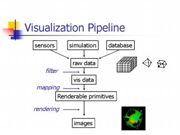
Visualization Pipeline
sensors
simulation
database
raw data
filter
vis data
mapping
Renderable primitives
rendering
images
2
Visualization Pipeline
sensors
simulation
database
raw data
- Denoising
- Decimation
- Multiresolution
- Mesh generation
- etc
filter
vis data
Renderable primitives
images
3
Visualization Pipeline
sensors
simulation
database
raw data
- Geometry
- Line
- Surface
- Voxel
- Attributes
- Color
- Opacity
- Texture
vis data
mapping
Renderable primitives
images
4
Visualization Pipeline
sensors
simulation
database
raw data
- Surface rendering
- Volume rendering
- Point based rendering
- Image based rendering
- NPR
vis data
Renderable primitives
rendering
images
5
Volume Rendering
- Goal visualize three-dimensional functions
- Measurements (medical imaging)
- Numerical simulation output
- Analytic functions
6
Data Representation
3D volume data are represented by a finite
number of cross sectional slices (a stack of
images)
N x 2D arraies 3D
array
7
Data Representation (2)
What is a Voxel? Two definitions
8
Important Steps
- Reconstruction
- Classification
- Optical model
- Shading
9
Reconstruction
- Recover the original continuous function from
discrete samples
10
Reconstruction
- Recover the original continuous function from
discrete samples
Box filter
Hat filter
Sinc filter
11
Classification
- Map from numerical values to visual attributes
- Color
- Transparency
- Transfer functions
- Color function c(s)
- Opacity function a(s)
12
Classification Order
- Pre classification Classification first, and
then filter - Post classification filter first, then
classification
25.3
post
pre
13
Optimal model
- Assume a density-emitter model (approximation)
- Each data point in the volume can emit and absorb
light - Light emission color classification
- Light absorption block light from behind due to
non-zero opacity
14
Optical Model
- Ray tracing is one method used to construct the
final image
x(t) ray, parameterized by t
s(x(t)) scalar value c(s(x(t)) color emitted
light a(s(x(t)) absorption coefficient
15
Ray Integration
- Calculate how much light can enter the eye for
each ray
16
Discrete Ray Integration
n
i-1
C S C (1- A )
i i
0
0
17
Shading
- Common shading model Phong model
- For each sample, evaluate
- C ambient diffuse specular
- constant Ip Kd (N.L) Ip Ks (N.H)
- Ip emission color at the sample
- N normal at the sample
i
n
18
Basic Idea
- Data are defined at the corners
- of each cell (voxel)
- The data value inside the
- voxel is determined using
- tri-linear interpolation
- No ray position round-off is
- needed when sampling
- Accumulate colors and opacities
- along the ray path
c1
c2
c3
19
Shading and Classification
- - Shading compute a color for each data point in
the - volume
- - Classification Compute an opacity for each
data point - in the volume
- Done by table lookup (transfer function)
- Levoy preshaded the entire volume
f(xi)
C(xi), a(xi)
20
Shading
- Use a phong illumination model
- Light (color) ambient diffuse specular
- C(x) Cp Ka Cp / (K1 K2 d(x))
- (Kd (N(x) . L Ks (N(x) . H )n
) - Cp color of light
- ka,kd,ks ambient, diffusive, specular
coefficient - K1,K2 constant (used for depth attenuation)
- N(x) normal at x
21
Normal estimation
- How to compute N(x)?
- Compute the gradient at each corner
- Interpolate the normal using central difference
N(x,y,z) (f(x1)-f(x-1))/2,
(f(y1)-f(y-1))/2,
(f(z1)-f(z-1))/2
Y1
z1
x-1,
y-1,
z-1
X1
22
Classification
Classification Mapping from data to opacities
Region of interest high
opaicity (more opaque) Rest
translucent or transparent The opacity function
is typically specified by the user Levoy 88
came up with two formula to compute opacity 1.
Isosurface 2. Region boundary (e.g.
between bone and fresh)
23
Opacity function (1)
- Goal visualize voxels that have a selected
threshold - value fv
- - No intermediate geometry is extracted
- - The idea is to assign voxels that have value fv
the - maximum opacity (say a)
- And then create a smooth transition for the
surrounding - area from 1 to 0
- Levoy wants to maintain a constant thickness for
the - transition area.
24
Opacity function (2)
Maintain a constant isosurface thickness
Can we assign opacity based on function value
instead of distance? (local operation we
dont know where the isosurface is) Yes we can
based on the value distance f fv
but we need to take into account the
local gradient
opacity a
opacity 0
25
Opacity function (3)
Assign opacity based on value difference (f-fv)
and local gradient gradient the value fall-off
rate grad Df/Ds Assuming a region has a
constant gradient and the isosurface transition
has a thickness R
F f(x) Then we interpolate the opacity opacity
a a ( fv-f(x))/ (grad R)
opacity a F fv
opacity 0 F fv grad R
thickness R
26
Continuous Sampling
- We sample the volume at discrete
- points along the ray
- (Levoy sampled color and opacity,
- but you can sample the value
- and then assign color and
- opacity)
- No integer round-off
- Use trilinear interpolation
- Compositing (front-to-back
- or back-to-front)
c1
c2
c3
27
Tri-linear Interpolation
- Use 7 linear interpolations
- Interpolate both value and
- gradient
- Levoy interpolate color and
- opacity
c2
28
Compositing
The initial pixel color Black Back-to-Front
compositing use under operator C C1
under background C C2 under C C C3 under
C Cout Cin (1-a(x)) C(x)a(x)
c1
c2
c3
29
Compositing (2)
Or you can use Front-to-Back Compositing
formula Front-to-Back compositing use over
operator C backgrond over C1 C C over C2
C C over C3 Cout Cin C(x)(1- ain)
aout ain a(x) (1-ain)
c1
c2
c3
30
Texture Mapping
Textured-mapped polygon
2D image
2D polygon
31
Tex. Mapping for Volume Rendering
Consider ray casting
(top view)
z
y
x
32
Texture based volume rendering
Use pProxy geometry for sampling
- Render every xz slice in the volume as a
texture-mapped polygon - The proxy polygon will sample the volume data
- Per-fragment RGBA (color and opacity) as
classification results - The polygons are blended from back to front
33
Texture based volume rendering
34
Changing Viewing Direction
What if we change the viewing position?
That is okay, we just change the eye position (or
rotate the polygons and re-render), Until
35
Changing View Direction (2)
Until
You are not going to see anything this way
This is because the view direction now is
Parallel to the slice planes What do we do?
36
Switch Slicing Planes
- What do we do?
- Change the orientation of slicing planes
- Now the slice polygons are parallel to
- YZ plane in the object space
37
Some Considerations (5)
When do we need to change the slicing
orientation?
When the major component of view vector changes
from y to -x
38
Some Considerations (6)
Major component of view vector? Given the view
vector (x,y,z) -gt get the maximal component If
x then the slicing planes are parallel to yz
plane If y then the slicing planes are parallel
to xz plane If z then the slicing planes are
parallel to xy plane -gt This is called
(object-space) axis-aligned method.
39
Three copies of data needed
- We need to reorganize the input textures for
diff. View directions. - Reorganize the textures on the fly is too time
consuming. We want to prepare the texture sets
beforehand
xz slices
yz slices
xy slices
40
Texture based volume rendering
Algorithm (using 2D texture mapping
hardware) Turn off the depth test Enable
blending For (each slice from back to front)
- Load the 2D slice of data into texture
memory - Create a polygon corresponding to
the slice - Assign texture coordinates to
four corners of the polygon - Render
and blend the polygon (use OpenGL alpha
blending) to the frame buffer
41
Problem (1)
- Non-even sampling rate
d
d
d
d gt d gt d
Sampling artifact will become visible
42
Problem (2)
Object-space axis-alighed method can create
artifact Popping Effect
There is a sudden change of slicing direction
when the view vector transits from one major
direction to another. The change in the image
intensity can be quite visible
43
Solution (1)
- Insert intermediate slides to maintain the
sampling rate
44
Solution (2)
Use Image-space axis-aligned slicing plane
the slicing planes are always parallel to the
view plane
45
3D Texture Based Volume Rendering
46
Image-Space Axis-Aligned
Arbitrary slicing through the volume and
texture mapping capabilities are needed
- Arbitrary slicing this can be computed
using software in real time
This is basically polygon-volume clipping
47
Image-Space Axis-Aligned (2)
Texture mapping to the arbitrary slices
This requires 3D Solid texture mapping Input
texture A bunch of slices (volume) Depending on
the position of the polygon, appropriate
textures are mapped to the polygon.
48
3D Texture Mapping
Now the input texture space is 3D Texture
coordinates (r,s) -gt (r,s,t)
(0,1,1)
(1,1,1)
(0,1,0)
(1,1,0)
(1,0,0)
(0,0,0)
49
Pros and Cons
- 2D textured object-aligned slices
- Very high performance
- High availability
- - High memory requirement
- - Bi-linear interpolation
- - inconsistent sampling rates
- - popping artifacts
50
Pros and Cons
- 3D textured view-aligned slices
- Higher quality
- No popping effect
- Need to compute the slicing planes for
- every view angle
- Limited availability (not anymore)
51
Classification Implementation
Red
v
Green
(R, G, B, A)
v
Blue
v
Alpha
value
v
52
Classification Implementation (2)
- Pre-classification using color palette
- glColorTableExt( GL_SHARED_TEXTURE_PALETTE_EXT,
GL_RGBA8, 2564, GL_RGBA, GL_UNSIGNED_BYTE,
color_palette) - Post-classification using 1D(2D,3D) texture
- glTexImage1D(Gl_TEXTURE_1D, 0, GL_RBGA8, 2564,
0, GL_RGBA, GL_UNSIGNED_BYTE, color_palette)
53
Classification implementation (3)
- Post-classification dependent texture
54
Shading
- Use per-fragment shader
- Store the pre-computed gradient into a RGBA
texture - Light 1 direction as constant color 0
- Light 1 color as primary color
- Light 2 direction as constant color 1
- Light 2 color as secondary color
55
Non-polygonal isosurface
- Store voxel gradient as GRB texture
- Store the volume density as alpha
- Use OpenGL alpha test to discard volume density
not equal to the threshold - Use the gradient texture to perform shading
56
Non-polygonal isosurface (2)
- Isosurface rendering results No shading
diffuse diffuse
specular
Recommended
CrystalGraphics Presentations


![Real-Time Volume Graphics [07] Global Volume Illumination PowerPoint PPT Presentation](https://s3.amazonaws.com/images.powershow.com/7513877.th0.jpg?_=20160105118)


