
Model and experiment setup - PowerPoint PPT Presentation
1 / 1
Title:
Model and experiment setup
Description:
Model and experiment setup. The Navy Coastal Ocean Model (NCOM) is used for ... The model domain is shown in Figure 1. The horizontal resolution is 1/60 . The ... – PowerPoint PPT presentation
Number of Views:48
Avg rating:3.0/5.0
Title: Model and experiment setup
1
Forced Tidal Response in the Gulf of Mexico
Flavien Gouillon1, Steven Morey1, Dmitry
Dukhovskoy1, James J. OBrien1,
(gouillon_at_coaps.fsu.edu)
1Center for Ocean-Atmospheric Predictions
Studies, Florida State University, Tallahassee,
FL, USA
Motivation Examination of the role of the
astronomical forcing in governing the behavior of
the tides and new tidal energetic estimates in
the Gulf of Mexico Introduction The present
study employs a non-assimilative numerical ocean
model to understand the nature of tides in the
Gulf of Mexico (GoM). A set of numerical
experiments is conducted to yield new
understanding of the tidal response due to a
local tidal potential, tidal signal propagation
coming from the Atlantic by considering forcing
at the model open boundaries, and the
modification of the propagating signal by
combining both model forcing mechanisms. Compariso
n of the model results with observations and
previous studies is conducted and new estimates
of total tidal power and tidal energy fluxes for
semidiurnal and diurnal constituents are produced
from the model.
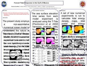
Tidal Energetics
Tidal amplitudes and phases
A set of new numerical experiments is run to
calculate tidal energy density maps, tidal power
and energy fluxes for M2 and O1. Figure 5 shows
the sum of the kinetic and potential energy per
unit area, averaged over the tidal constituent
period. Prominent features include an area of
weak energy spatially corresponding with the
amphidrome, which naturally has a zero elevation
through time. The maximum energy is found to be
at the shelf and confirms the tidal shelf
amplification theory. Contours show that the two
forcing mechanisms work constructively together
to increase the tidal signal in some regions as
well as destructively interfering to decrease the
tidal elevation in other area. For O1, the energy
density map is spatially uniform due mainly to
the co-oscillating phenomena. Table 1 gives the
M2 and O1 tidal power within the Gulf for each
experiments. Energy fluxes are computed according
to Kowalik 1993 and are given by
(2) These fluxes are shown in Figure
6. The net tidal energy dissipation and their
comparison with previous studies are given by the
Table 2
- The sea surface elevation time series from each
model experiment is analyzed using the T-Tide
Pawlowiscz et al, 2002 harmonic analysis
utility to extract estimates of the phases and
amplitude. Resulting maps are shown in Figure 2.
Results for semidiurnal constituents are describe
in part a) and diurnal constituents description
are in part b). Figure 3 and 4 compare amplitudes
and phases to observations from the tidal gauges
shown in Figure 1. - a) The LTPOB experiment (Figure 2a) shows a good
agreement with previous studies. For the
semidiurnal constituent the amphidromic point is
north of the Yucatan Peninsula (YP). The co-tidal
lines become compacted in the central GoM,
roughly following a line from the U.S. Gulf Coast
to the YP. This is where the tidal pattern
changes to become predominantly diurnal. The
maximal tidal amplitudes are found in the wide
shelves due to resonance phenomena Clarke,
1995. Considering only the OB forcing (Figure
2b), the amphidromic point is slightly shifted to
the northeast and the tidal wave is traveling
faster. - b) The LTPOB experiment for the diurnal
experiment (Figure 2c) shows that phases are very
uniform into the basin. Both entrances are at the
same phase which show the co-oscillating
phenomena. Combining the LTP forcing does not
change the behavior of the diurnal tides (Figure
2d) except a slight decrease on the overall
amplitude which will have an impact on the total
diurnal tidal energy in the basin.
b)
Model and experiment setup The Navy Coastal
Ocean Model (NCOM) is used for numerical
simulation of the sea level response to tidal
forcing. The NCOM is a three-dimensional ocean
model but In these simulations, it is run as a
barotropic ocean model. The model domain is shown
in Figure 1. The horizontal resolution is 1/60.
The model Open Boundaries (OB) are the Straits of
Florida and the Caribbean Sea (Figure 1). Flather
1976 OB conditions are applied. The basin is
initially at rest and there is no forcing but
tides. Only the main four tidal constituents are
considered (M2, S2, O1, K1) in this study as they
represent 90 of the total tidal bulk He and
Weisberg, 2002. Only M2 and O1 are shown
here. Three model experiments are
performed 1) Model forced by a local tidal
potential given by equation (1) and derived from
Newtons tidal theory (LTP
experiment)
(1) 2) Model forced only at
OB by tidal barotropic transport and velocities
derived from the western Atlantic ADCIRC
model Mukai et al, 2002 (OB experiment) 3)
Both forcing mechanisms are combined (LTPOB
experiment)
Figure 1 Model domain and
tidal gauges Figure 1 Model
domain and tidal gauges
Figure 5 Total energy density maps (colored on a
logarithmic scale, units are J.m-2). Contours
are the ratios of the tidal energy density for
the LTP (black solid line) and OB (gray dashed
line) over the tidal energy density of the LTPOB
experiment for M2 (left panel) and O1 (right
panel).
d)
Figure 2 Tidal amplitudes in meters (contoured)
and phases in degrees (colored) for all tidal
constituents. OB experiment is left panel and
LTPOB is right panel.
Figure 6 Energy fluxes in the GoM
Table 1 Tidal power in GW
Table 2 Net tidal energy dissipation in GW
Conclusion The LTP forcing alters the tidal
signal propagating from the model OB especially
for the semidiurnal constituent. The astronomical
forcing needs to be taken into account for high
resolution numerical studies of the GoM. A
careful tidal energetic study provides new
estimates of tidal power and tidal dissipation
rates within the GoM and confirms that the GoM is
acting as a major sink for both semidiurnal as
well as diurnal tidal energy.
Clarke, Allan J., (1995), Northeastern Gulf of
Mexico physical oceanography workshop 417
proceedings of a workshop held in Tallahassee,
Florida, April 5-7, 1994. Prepared by 418 Florida
State University. OCS Study MMS 94-0044. U.S.
Department of the Interior, 419 Minerals
Management Services, Gulf of Mexico OCS Region,
New Orleans, La. 420 257pp. Flather, R.A.,
(1976), A tidal model of the northwest European
continental shelf. 425 Memoires de la societe
Royale de Liege 6 (10), 141-162. Gouillon F., S.
M. Morey, D. S. Dukhovskoy, J.J. OBrien (2007),
Forced Tidal response in the Gulf of Mexico,
Journ. Geophys. Res, In Review.
Figure 3 Comparison of tidal phases
Figure 4 Comparison of tidal amplitudes
Recommended
CrystalGraphics Presentations


