AP Physics Mechanics for Physicists and Engineers Agenda for Today

1
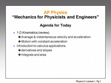
AP Physics Mechanics for Physicists and
EngineersAgenda for Today

• 1-D Kinematics (review).
• Average instantaneous velocity and acceleration
• Motion with constant acceleration
• Introduction to calculus applications
• derivatives and slopes
• Integrals and area

2
Kinematics Problems

• 1-D Kinematics
• Average instantaneous velocity (Chapter2
  1,4,5,11-13,15-17) and acceleration (18,21)
• Motion with constant acceleration(23,24,27,31,35,3
  7,39,40-1,43)
• Free Fall (44,47,49,51,53,56,61,63)
• Motion Graphs (66,67,69,70)
• Review Phun!!

3
Kinematics

• Location and motion of objects is described using
  Kinematic Variables
• Some examples of kinematic variables.
• position r vector
• velocity v vector
• Kinematic Variables
• Measured with respect to a reference frame. (x-y
  axis)
• Measured using coordinates (having units).
• Many kinematic variables are Vectors, which means
  they have a direction as well as a magnitude.
• Vectors denoted by boldface V or arrow

4
Motion in 1 dimension
See text 2-1

• In general, position at time t1 is usually
  denoted r(t1).
• In 1-D, we usually write position as x(t1 ).
• Since its in 1-D, all we need to indicate
  direction is or ?.
• Displacement in a time ?t t2 - t1 is
  ?x x(t2 ) - x(t1 ) x2 - x1

x
some particles trajectoryin 1-D
x2
??x
x1
t
t1
t2
??t
5
1-D kinematics
See text 2-1

• Velocity v is the rate of change of position
• Average velocity vav in the time ??t t2 - t1
  is

x
trajectory
x2
??x
Vav slope of line connecting x1 and x2.
x1
t
t1
t2
??t
6
1-D kinematics...
See text 2-2

• Instantaneous velocity v is defined as

x
so V(t2 ) slope of line tangent to path at t2.
x2
??x
x1
t
t1
t2
??t
7
1-D kinematics...
See text 2-3

• Acceleration a is the rate of change of
  velocity
• Average acceleration aav in the time ??t t2
  - t1 is

• And instantaneous acceleration a is defined as

8
Recap

• If the position x is known as a function of time,
  then we can find both velocity v and acceleration
  a as a function of time!

x
t
v
t
a
t
9
More 1-D kinematics

• We saw that v ?x / ?t
• so therefore ?x v ?t ( i.e. 60 mi/hr x 2 hr
  120 mi )
• In calculus language we would write dx v dt,
  which we can integrate to obtain

• Graphically, this is adding up lots of small
  rectangles

v(t)

...
displacement
t
10
1-D Motion with constant acceleration
See text 2-4

• High-school calculus
• Also recall that
• Since a is constant, we can integrate this using
  the above rule to find
• Similarly, since we can
  integrate again to get

11
Recap
See text Table 2-1 (p. 33)

• So for constant acceleration we find

x
t
v

• From which we can derive

t
a
t
12
Problem 1

• A car traveling with an initial velocity vo. At
  t 0, the driver puts on the brakes, which slows
  the car at a rate of ab

13
Problem 1...

• A car traveling with an initial velocity vo. At
  t 0, the driver puts on the brakes, which slows
  the car at a rate of ab. At what time tf does
  the car stop, and how much farther xf does it
  travel ??

vo
ab
x 0, t 0
v 0
x xf , t tf
14
Problem 1...

• Above, we derived (a)
  (b)
• Realize that a -ab
• Using (b), realizing that v 0 at t tf
• find 0 v0 - ab tf or tf vo /af
• Plugging this result into (a) we find the
  stopping distance

15
Problem 1...

• So we found that
• Suppose that vo 65 mi/hr x .45 m/s / mi/hr
  29 m/s
• Suppose also that ab g 9.8 m/s2.
• Find that tf 3 s and xf 43 m

16
Tips

• Read !
• Before you start work on a problem, read the
  problem statement thoroughly. Make sure you
  understand what information in given, what is
  asked for, and the meaning of all the terms used
  in stating the problem.
• Watch your units !
• Always check the units of your answer, and carry
  the units along with your numbers during the
  calculation.
• Understand the limits !
• Many equations we use are special cases of more
  general laws. Understanding how they are derived
  will help you recognize their limitations (for
  example, constant acceleration).

17
Recap of kinematics lectures

• 1-D Kinematics
• Average instantaneous velocity (Chapter3-
  1,3,7,9,11) and and acceleration
• Motion Graphs (14,15,17,19)
• Motion with constant acceleration(Ch3
  21,23,27,29,31,35,37 41)
• Free Fall (Ch3-41,43,47,49,51,52)
• Review Phun!! (67,69,70 )