Object Recognition using Invariant Local Features

1
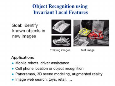
Object Recognition using Invariant Local Features
Goal Identify known objects in new images
Training images Test image

• Applications
• Mobile robots, driver assistance
• Cell phone location or object recognition
• Panoramas, 3D scene modeling, augmented reality
• Image web search, toys, retail,

2
Local feature matchingTorr Murray (93) Zhang,
Deriche, Faugeras, Luong (95)

• Apply Harris corner detector
• Match points by correlating only at corner points
  
• Derive epipolar alignment using robust
  least-squares

3
Rotation InvarianceCordelia Schmid Roger Mohr
(97)

• Apply Harris corner detector
• Use rotational invariants at corner points
• However, not scale invariant. Sensitive to
  viewpoint and illumination change.

4
Scale-Invariant Local Features

• Image content is transformed into local feature
  coordinates that are invariant to translation,
  rotation, scale, and other imaging parameters

SIFT Features
5
Advantages of invariant local features

• Locality features are local, so robust to
  occlusion and clutter (no prior segmentation)
• Distinctiveness individual features can be
  matched to a large database of objects
• Quantity many features can be generated for even
  small objects
• Efficiency close to real-time performance
• Extensibility can easily be extended to wide
  range of differing feature types, with each
  adding robustness

6
Build Scale-Space Pyramid

• All scales must be examined to identify
  scale-invariant features
• An efficient function is to compute the
  Difference of Gaussian (DOG) pyramid (Burt
  Adelson, 1983)

7
Scale space processed one octave at a time
8
Key point localization

• Detect maxima and minima of difference-of-Gaussian
  in scale space

9
Sampling frequency for scale
More points are found as sampling frequency
increases, but accuracy of matching decreases
after 3 scales/octave
10
Select canonical orientation

• Create histogram of local gradient directions
  computed at selected scale
• Assign canonical orientation at peak of smoothed
  histogram
• Each key specifies stable 2D coordinates (x, y,
  scale, orientation)

11
Example of keypoint detection
Threshold on value at DOG peak and on ratio of
principle curvatures (Harris approach)

• (a) 233x189 image
• (b) 832 DOG extrema
• (c) 729 left after peak
• value threshold
• (d) 536 left after testing
• ratio of principle
• curvatures

12
SIFT vector formation

• Thresholded image gradients are sampled over
  16x16 array of locations in scale space
• Create array of orientation histograms
• 8 orientations x 4x4 histogram array 128
  dimensions

13
Feature stability to noise

• Match features after random change in image scale
  orientation, with differing levels of image
  noise
• Find nearest neighbor in database of 30,000
  features

14
Feature stability to affine change

• Match features after random change in image scale
  orientation, with 2 image noise, and affine
  distortion
• Find nearest neighbor in database of 30,000
  features

15
Distinctiveness of features

• Vary size of database of features, with 30 degree
  affine change, 2 image noise
• Measure correct for single nearest neighbor
  match

16
Detecting 0.1 inliers among 99.9 outliers

• We need to recognize clusters of just 3
  consistent features among 3000 feature match
  hypotheses
• RANSAC would be hopeless!
• Generalized Hough transform
• Vote for each potential match according to model
  ID and pose
• Insert into multiple bins to allow for error in
  similarity approximation
• Check collisions

17
Probability of correct match

• Compare distance of nearest neighbor to second
  nearest neighbor (from different object)
• Threshold of 0.8 provides excellent separation

18
Model verification

1. Examine all clusters with at least 3 features
2. Perform least-squares affine fit to model.
3. Discard outliers and perform top-down check for
   additional features.
4. Evaluate probability that match is correct

19
3D Object Recognition

• Extract outlines with background subtraction

20
3D Object Recognition

• Only 3 keys are needed for recognition, so extra
  keys provide robustness
• Affine model is no longer as accurate

21
Recognition under occlusion
22
Test of illumination invariance

• Same image under differing illumination

273 keys verified in final match
23
Examples of view interpolation
24
Recognition using View Interpolation
25
Location recognition
26
Robot localization results

• Joint work with Stephen Se, Jim Little

• Map registration The robot can process 4
  frames/sec and localize itself within 5 cm
• Global localization Robot can be turned on and
  recognize its position anywhere within the map
• Closing-the-loop Drift over long map building
  sequences can be recognized. Adjustment is
  performed by aligning submaps.

27
Robot Localization
28
(No Transcript)
29
Map continuously built over time
30
Locations of map features in 3D
31

• Sony Aibo
• (Evolution Robotics)
• SIFT usage
• Recognize
• charging
• station
• Communicate
• with visual
• cards