
Reprise: dirty beam, dirty image' - PowerPoint PPT Presentation
1 / 25
Title:
Reprise: dirty beam, dirty image'
Description:
Fourier inversion of V times the sampling function S gives the dirty image ID: ... Merlin, d= 35 eMerlin, d= 35 Narrow vs broad-band: UV coverage ... – PowerPoint PPT presentation
Number of Views:50
Avg rating:3.0/5.0
Title: Reprise: dirty beam, dirty image'
1
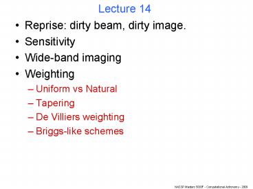
Lecture 14
- Reprise dirty beam, dirty image.
- Sensitivity
- Wide-band imaging
- Weighting
- Uniform vs Natural
- Tapering
- De Villiers weighting
- Briggs-like schemes
2
Reprise dirty beam, dirty image.
- Fourier inversion of V times the sampling
function S gives the dirty image ID - This is related to the true sky image I by
- The dirty beam B is the FT of the sampling
function - (Can get B by setting all the V to 1, then FT.)
3
Reprise l and m
- Remember that l sin ?. ? is the angle from the
phase centre. - For small l, l ? (in radians of course).
- m is similar but for the orthogonal direction.
Direction of phase centre.
Direction of source.
l
?
4
Sensitivity
- Image noise standard deviation (for the
weak-source case) is (for natural weighting) - N here is the number of antennas.
- Note that Ae is further decreased by correlator
effects for example by 2/p if 1-bit
digitization is used. - Actual sensitivity (minimum detectable source
flux) is different for different sizes of source. - Due to the absence of baselines lt the minimum
antenna separation, an interferometer is
generally poor at imaging large-scale structure.
5
Wide-band imaging.
How can we increase UV coverage?we could get
more baselines if we moved the antennas!
6
but it is simpler to change the observing
wavelength.
?
eg
?/2
7
With many wavelengths
we have many baselines,
and, effectively,
many antennas.
8
Narrow vs broad-band UV coverage
16 x 1 MHz
2000 x 1 MHz
Merlin, d35
eMerlin, d35
9
Narrow vs broad-band - without noise
16 x 1 MHz
2000 x 1 MHz
10
Narrow vs broad-band - with noise
16 x 1 MHz
2000 x 1 MHz
SNR of each visibility 15.
11
Weighting or how to shape the dirty beam.
- Why should we weight the visibilities before
transforming to the sky plane? - Because the uneven distribution of samples of V
means that the dirty beam has lots of ripples or
sidelobes, which can extend a long way out. - These can hide fainter sources.
- Even if we can subtract the brighter sources,
there are always errors in our knowledge of the
dirty beam shape. - If there must be some residual, the smoother and
lower it is, the better.
12
Weighting
- There are usually far more short than long
baselines.
The distribution of baselines also nearly always
has a hole in the middle.
Baseline length
13
Weighting
- A crude example
This bin has 1 sample.
This bin has 84 samples.
14
Weighting
- What do we get if we leave the visibilities
alone? - The resulting dirty beam will be broad (? low
resolution), because there are so many more
visibility samples at small (u,v) than large
(u,v). - BUT, if the uncertainties are the same for every
visibility, leaving them unweighted (ie, all
weights Wj,k1) gives the lowest noise in the
image. - This is called natural weighting.
- The easiest other thing to do is set Wj,k1/(the
number of visibilities in the j,kth grid cell). - This is called uniform weighting.
- Then optionally multiply everything by a
Gaussian - Called tapering.
15
Natural vs uniform
Natural weighting
Uniform weighting
16
The resulting dirty images
Natural weighting
Uniform weighting
17
But if we add in some noise...
Natural weighting
Uniform weighting
SNR of each visibility 0.7.
18
Tradeoff
- This sort of tradeoff, between increasing
resolution on the one hand and sensitivity on the
other, is unfortunately typical in interferometry.
19
Some other recent ideas
- Scheme by Mattieu de Villiers (new, not yet
published SA work) - Weight by inverse of density of samples.
- My own contribution
- Iterative optimization. Has the effect of
rounding the weight distribution to feather out
sharp edges in the field of weights. - Havent got the bugs out of it yet.
Ideal smooth weight function (Fourier inverse of
desired PSF)
Densely packed samples are down-weighted.
Isolated samples get weighted higher so that the
average approaches the ideal.
20
Weighting schemes
Simulated e-Merlin data. 400 x 5 MHz
channels ?av 6 GHz tint 10 s d 30
Iterative best fit out- side 20-pixel radius
Uniform
Tapered uniform
21
Dirty beam images (absolute values).
Iterative best fit out- side 20-pixel radius
Uniform
Tapered uniform
22
Comparison slices through the DIs
Natural (narrow-band)
Natural
Uniform
Optimized for rgt10
23
More on iterated weights
r 10
24
But real data is noisy
SNR of each visibility 5.
25
One could think of other feathering schemes.
- Multiply visibilities
- with a vignetting
- function of time and
- frequency, eg
2. Aips task IMAGR parameter UVBOX effectively
smooths the weight function. See also D
Briggs PhD thesis.
Recommended
CrystalGraphics Presentations


