
Linear and Quadratic Functions - PowerPoint PPT Presentation
1 / 40
Title:
Linear and Quadratic Functions
Description:
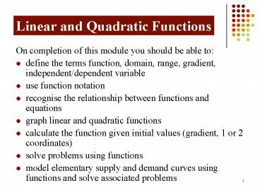
Linear and Quadratic Functions On completion of this module you should be able to: define the terms function, domain, range, gradient, independent/dependent variable – PowerPoint PPT presentation
Number of Views:369
Avg rating:3.0/5.0
Title: Linear and Quadratic Functions
1
Linear and Quadratic Functions
- On completion of this module you should be able
to - define the terms function, domain, range,
gradient, independent/dependent variable - use function notation
- recognise the relationship between functions and
equations - graph linear and quadratic functions
- calculate the function given initial values
(gradient, 1 or 2 coordinates) - solve problems using functions
- model elementary supply and demand curves using
functions and solve associated problems
2
Functions
A function describes the relationship that exists
between two sets of numbers. Put another way, a
function is a rule applied to one set of numbers
to produce a second set of numbers.
3
Example Converting Fahrenheit to Celsius
This rule operates on values of F to produce
values of C.
The values of F are called input values and the
set of possible input values is called the domain.
The values of C are called output values and the
set of output values produced by the domain is
called the range.
4
Function Notation
Consider the function
The x are the input values and f(x), read f of x,
are the output values.
The domain is the set of positive real numbers
including 0 and excepting 3. (Why?) The output
values produced by the domain is the range.
Sometimes the symbol y is used instead of f(x).
5
Function and Equations
An equation is produced when a function takes on
a specific output value.
eg f(x) 3x 6 is a function.
When f(x) 0, then the equation becomes
0 3x 6 which can be easily solved
(to give x -2)
6
This is shown graphically as follows
7
Graphing Functions
Input and output values form coordinate pairs
(x, f(x)) or (x, y).
x values measure the distance from the origin in
the horizontal direction and f(x) values the
distance from the origin in the vertical
direction.
To plot a straight line (linear function), 2 sets
of coordinates (3 sets is better) must be
calculated. For other functions, a selection of
x values should be made and coordinates
calculated.
8
Example Linear Function
Graph f(x) 2x - 4
9
(No Transcript)
10
Example Quadratic Function
Graph the function
At the y-intercept, x 0, so and the
coordinate is (0,2).
11
At the x-intercept, f(x) 0, so and the
coordinates are (2,0) and (0.5,0).
12
Vertex
The coordinates of the vertex are (1.25, -1.125).
13
2
(0,2)
(0.5,0)
1
2
(2,0)
x
-1
(1.25, -1.125)
14
Linear Functions
- All linear functions (or equations) have the
following features - a slope or gradient (m)
- a y-intercept (b)
- If (x1, y1) and (x2, y2) are two points on the
line then the gradient is given by
15
- Gradient is a measure of the steepness of the
line. - If m gt 0, then the line rises from left to
right. - If m lt 0, the line falls from left to right.
- A horizontal line has a gradient of 0 a
vertical line has an undefined gradient. - The y-intercept is calculated by substituting
x 0 into the equation for the line.
16
All straight line functions can be expressed in
the form y mx b Note The
standard form equation for linear functions is Ax
By C 0. Equations in this form are not as
useful as when expressed as y mx
b. Equations can be derived in the following
way, depending on what information is given.
17
Deriving Straight Line Functions
- Given (x1, y1) and (x2, y2)
- Given m and (x1, y1)
- Given m and b
18
Problem Depreciation
A tractor costs 60,000 to purchase and has a
useful life of 10 years. It then has a scrap
value of 15,000. Find the equation for the
book value of the tractor and its value after 6
years.
19
V
60,000
?
15,000
t
6
10
20
Value (V) depends on time (t). t is called the
independent variable and V the dependent
variable. The independent variable is always
plotted on the horizontal axis and the dependent
variable on the vertical axis.
21
Given two points, the equation becomes
22
or more correctly
The book value of the tractor after 6 years is
33,000.
23
Example
Suppose a manufacturer of shoes will place on the
market 50 (thousand pairs) when the price is 35
(per pair) and 35 (thousand pairs) when the price
is 30 (per pair). Find the supply equation,
assuming that price p and quantity q are linearly
related.
24
(No Transcript)
25
The supply equation is
26
Example
For sheep maintained at high environmental
temperatures, respiratory rate r (per minute)
increases as wool length l (in centimetres)
decreases. Suppose sheep with a wool length of
2cm have an (average) respiratory rate of 160,
and those with a wool length of 4cm have a
respiratory rate of 125. Assume that r and l are
linearly related. (a) Find an equation that gives
r in terms of l. (b) Find the respiratory rate of
sheep with a wool length of 1cm.
27
(a) Find r in terms of l ? l is independent
r is dependent Coordinates will be of the
form (l, r).
28
(No Transcript)
29
(b) When l 1
When wool length is 1 cm, average respiratory
rate will be 177.5 per minute.
30
Quadratic Functions
All quadratic functions can be written in the
form where a, b and c are constants and a ? 0.
31
Elementary Supply and Demand
In general, the higher the price, the smaller the
demand is for some item and as the price falls
demand will increase.
p
Demand curve
q
32
Concerning supply, the higher the price, the
larger the quantity of some item producers are
willing to supply and as the price falls, supply
decreases.
p
Supply curve
q
33
Note that these descriptions of supply and demand
imply that they are dependent on price (that is,
price is the independent variable) but it is a
business standard to plot supply and demand on
the horizontal axis and price on the vertical
axis.
34
Example Equilibrium price
The supply of radios is given as a function of
price by and demand by Find the equilibrium
price.
35
Graphically, Note the restricted domains.
70
equilibrium price
0
p
1
2
3
4
5
0
36
Algebraically, D(p) S(p)
37
-14 is not in the domain of the functions and so
is rejected. The equilibrium price is 4.
38
Example Maximising profit
If an apple grower harvests the crop now, she
will pick on average 50 kg per tree and will
receive 0.89 per kg. For each week she waits,
the yield per tree increases by 5 kg while the
price decreases by 0.03 per kg. How many weeks
should she wait to maximise sales revenue?
39
Weight and Price can both be expressed as
functions of time (t). W(t) 50 5t P(t)
0.89 - 0.03t
40
Maximum occurs at
She should wait 9.83 weeks ( 10 weeks) for
maximum revenue. (R 59 per tree)