V24 Hybrid-methods for macromolecular complexes

1
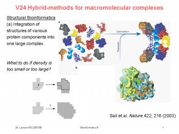
V24 Hybrid-methods for macromolecular complexes
Structural Bioinformatics (a) Integration of
structures of various protein components into one
large complex. What to do if density is too
small or too large?

Sali et al. Nature 422, 216 (2003)
2
Correlation-based fitting

Correlation-mapping can also be used to position
small fragments into large templates. As shown
before it can also be adapted to accomodate
molecular flexibility during fitting.
Wriggers, Chacon, Structure 9, 779 (2001)
3
Aim Accelerated Correlation-Based Fitting with
FFT
The initial data sets are a low-resolution map
(target) and an atomic structure (probe),
corresponding to direct space densities ?em(r)
and ?atomic(r), respectively (blue box). The
probe molecule is subject to a rotation matrix R
(red box) that can be constructed from the three
Euler angles. After lowering the resolution of
the atomic structure (by direct space convolution
with a Gaussian g) to that of the target map, the
rotated probe molecule corresponds to the
simulated density ?calc(r). An optional filter e
(e.g., a Laplacian) can be applied to both ?em
(r) and ?calc(r) before the structure factors are
computed (f denotes the FFT and the asterisk
denotes the complex conjugate).

The definition of a direct space convolution of a
density function b(r) with a kernel a(r) is given
in the green box. The definition of the direct
space correlation C as a function of a
translational displacement T is given in the
orange box. By virtue of the Fourier correlation
theorem, C can be computed for all T from the
inverse Fourier transform of the previously
calculated structure factors.
Wriggers, Chacon, Structure 9, 779 (2001)
4
Matching densities
Intuitively, we want to compute the overlap of
the two densities after placing the two lattices
on top of each other. But what means 'on top of
each other' in mathematical terms?

Orienting the two lattices can be done with
respect to 6 degrees of freedom, 3 for
translation along x, y, and z, and 3 for
rotation around the angles ?, ?, and ?. Among
all these possibilities, one wishes to identify
the relative orientation x, y, z, ?, ?, ? that
minimizes the sum of least squares Here, R?,?,?
is a three-dimensional rotation matrix and Tx,y,z
is a translation operator that translates
molecule B to the position x, y, z. Minimizing
the sum of squared errors is equivalent to
maximizing the linear cross-correlation of A and
B, for a given translation vector (x,y,z)
and rotation (?, ?, ?).
5
Situs package Automated low-resolution fitting

• The data sets need to be compared at comparable
  resolution
• project atomic structure B on the cubic lattice
  of the EM data A
• by tri-linear interpolation, and convolute each
  lattice points bl,m,n with a Gaussian function g.

The complexity of computing this correlation for
all translations and rotations in direct space
is O(N6).
Chacon, Wriggers J Mol Biol 317, 375 (2002)
6
Laplacian filter for edge enhancement
In the absence of hard boundaries, the contour of
a low-resolution object is contained in the 3D
edge information instead of a 2D surface. A
simple and computationally cheap filter for 3D
edge enhancement is the Laplacian filter
that approximates the Laplace operator of the
second derivative. Applied to the density
gradient on a grid, the Laplacian filtered
density can be quickly computed by a finite
difference scheme
where aijk and ?2aijk represent the density and
the Laplacian filtered density at grid point
(i,j,k). The expression compares the values at
grid points 1 and -1 along all three directions
to the value of the grid point ijk.
7
Schematic view of a Laplacian filter
ai-1jk, aijk, and ai1jk are the density values
at three neighboring grid points in one
direction. The grey lines denote the difference
between the central point and the values to the
left and to the right. These are finite
difference approximations of the first derivative
left and right of the grid point ijk. The dotted
line and dotted arrow illustrate how the two
first derivatives are combined to obtain an
approximation of the second derivative at grid
point ijk by finite difference as ai1jk ai-1jk
-2 aijk.
8
Effect of Laplacian filter
Include surface information in the volume
docking procedure. Laplacian filter

Effect of Laplacian filter Left cross-section
of 15Å simulated density of RecA hexameric
structure. Right same density after application
of Laplacian filter. Secondary derivatives are
maximal here because signal increases in various
directions.
Chacon, Wriggers J Mol Biol 317, 375 (2002)
9
Efficient evaluation of correlation by FFT
Geometric match between two molecules A and B can
be measured by the Laplacian cross-correlation

6D rigid-body search has complexity N6. Common
problem in protein-ligand and in protein-protein
docking. Efficient solution (Katchalski-Kazir
algorithm) use FFT because FFT has complexity
N3logN3 ?
Chacon, Wriggers J Mol Biol 317, 375 (2002)
10
Situs package success case
Fitting of tubulin components to an experimental
20Å resolution map of microtubuli. Without any a
priori consideration about the relative
orientation of ? and ? tubulins, the atomic
structure of the ??-tubulin dimer could be
reconstructed to within 2Å of the known dimer
X-ray structure (labeled by Nogales et al.).

Chacon, Wriggers J Mol Biol 317, 375 (2002)
11
Core-weighted fitting Grid-threading
Monte-Carlo
Idea define core region of a structure as the
part whose density distribution is unlikely to be
altered by the presence of adjacent
components. Surface region is accessible/may
interact with other components. Use again
Laplacian filter defined by a finite difference
approximation to define the boundary of the
surface where aijk and ?2aijk represent the
density and the Laplacian filtered density at
grid point (i,j,k).

Wu, Milne, .., Subramaniam, Brooks, J Struct Biol
141, 63 (2003)
12
Core-weighted fitting I core index
Define core index, which describes the depth of a
grid point located within this core where
fijk is the core index of grid point (i,j,k), ac
is a cutoff density minfi?1jk, fij?1k ,fijk?1
represents the minimum core index of the
neighboring grid points around grid point (i,j,k).

Wu, Milne, .., Subramaniam, Brooks, J Struct Biol
141, 63 (2003)
13
Core-weighted fitting I core index
The core index is zero for grid points outside
the core and increases progressively for grid
points located deeper in the core. A grid point
outside the core region must neighbor at least
one grid point that is also outside the core. A
grid point within the core cannot neighbor a grid
point outside the core unless it satisfies the
condition ?2aijk ? 0 and aijk gt ac.

• Use this iterative procedure for calculating the
  core incex
• initialize core index so that all core indices
  are 1 except the grid points at the boundary
• loop over all grid points
• repeat (b) until all grid points satisfy equation
  on p.31.

Wu, Milne, .., Subramaniam, Brooks, J Struct Biol
141, 63 (2003)
14
Core indices for 2 proteins and their complex
Grid points labelled by value of core
index. Regions of protein density are colored
grey. For both proteins, the core index is 0
outside the domains, 1 at the outer edge and
becomes larger inside the proteins. Bold numbers
indicate the core indices of proteins A and B
that change upon formation of the AB complex.

Wu, Milne, .., Subramaniam, Brooks, J Struct Biol
141, 63 (2003)
15
Core-weighted correlation function
The match in density between two maps is again
described by a density correlation function (DC)

m and n refer to the two maps being compared,
and
represent the average and fluctuation of the
density fluctuation. Alternativey, one can use
the Laplacian correlation (LC)
Wu, Milne, .., Subramaniam, Brooks, J Struct Biol
141, 63 (2003)
16
Core-weighted fitting I core index - properties

• We expect the following features when we consider
  the match between the map of an individual
  component and the map of a multicomponent
  assembly
• If the core region of an individual component
  matches the core region of the complex, the
  distribution property of this core region should
  not change appreciably for the correct fit.
• If the surfaces match, the distribution property
  of this surface region should not change
  appreciably for the correct fit.
• If the surface (low core index) of an individual
  component matches the core (high core index) of
  the complex, the distribution property of the
  surface region should change significantly for
  the correct fit.
• If the core (high core index) of an individual
  component matches the surface (low core index) of
  the complex, it cannot be a correct fit.
• A correlation function works fine for scenarios
  1, 2, and 4 to distinguish the correct fit from
  wrong fits.

Wu, Milne, .., Subramaniam, Brooks, J Struct Biol
141, 63 (2003)
17
Core-weighted fitting I core index - algorithm

• one needs to minimize the contribution from
  scenario 3 in the correlation function
  calculation. Can be achieved by down-weighting
  such matches.
• Use

• where wmn is the core-weighting function for the
  individual component m to the complex n. a, b, c
  are suitable parameters.
• core-weighted correlation function
• where represents a core-weighted
  average of property X

and
Wu, Milne, .., Subramaniam, Brooks, J Struct Biol
141, 63 (2003)
18
Core-weighted fitting I core index - algorithm
If we choose densities for the calculation, we
obtain the core-weighted density correlation
(CWDC)

and if we choose to apply the Laplacian filter,
we obtain the core-weighted Laplacian correlation
(CWLC)
The core-weighted correlation functions are
designed to down-weight the regions overlapping
with other components, while emphasizing the
regions with no overlap.
Wu, Milne, .., Subramaniam, Brooks, J Struct Biol
141, 63 (2003)
19
Grid-threading Monte-Carlo
Shown on the right is a grid-threading Monte
Carlo search in 2D. It is a combination of a grid
search and a Monte Carlo sampling. The
conformational space is divided into a 33 grid.
From each of the 9 grid points, short MC searches
(shown as purple curves) are performed to locate
a nearby local maximum. The global maximum is
identified from among these local maxima. Only
conformations along the 9 Monte Carlo paths are
searched.

Wu, Milne, .., Subramaniam, Brooks, J Struct Biol
141, 63 (2003)
20
Algorithm

• For a protein component, divide 6D search space
  to provide initial conformational states covering
  the whole space
• nx ? ny ? nz for translational sampling
• n? ? n? ? n? for rotational sampling
• Perform MC search starting from each grid point
  over NMC steps. At each move the component is
  translated along a random vector (xr, yr, zr) and
  then rotated around x,y,z axes for random angles
  (?r,?r,?r).
• A trial move is accepted if
• and rejected otherwise.
• T is a reduced temperature.

Wu et al. J Struct Biol 141, 63 (2003)
21
Algorithm

• Nonoverlapping local maxima are stored in
• sorted, linked list. Step (2) is repeated until
• all grid points are searched
• Identify global maximum from linked list and
• assign to component.
• Repeat steps (1) to (4) until all components
• have been fitted into the density map.

Wu et al. J Struct Biol 141, 63 (2003)
22
Test of Core-weighting method
(a) The X-ray structure of TCR variable domain
(PDB code 1A7N) and a 15 Å map generated from
the structure using pdblur from Situs. (b) The ?
-chain (red) at the maximum density correlation
position. The ?-chain is at its X-ray position
for reference.

Observation DC identifies wrong global maximum
for this 15 Å map. Other methods are more stable
at lower resolutions (see table).
Wu et al, J Struct Biol 141, 63 (2003)
23
Performance of systematic sampling

• The maximum core-weighted density correlations
  between the map of TCR
• ?-chain and the map of the TCR ?? complex
  identified from grid searches of the 6D
  conformational space (n6 grid points). 15 Å
  resolution maps.
• Black dashed line correlation value for the
  X-ray coordinates.
• An exponential increase in grid sampling size is
  required to improve the correlation values.
• grid searches are computationally inefficient.

Wu, Milne, .., Subramaniam, Brooks, J Struct Biol
141, 63 (2003)
24
Performance of grid search and Monte Carlo
The core-weighted density correlation function as
before during Monte Carlo searches starting from
each of the 26 grid points. The Monte Carlo
searches were performed with max15 Å, max30,
and T0.01. Each line represents one Monte Carlo
search procedure. The ability to converge to the
correct fit and the speed of convergence depend
significantly on the starting position.

Useful strategy identify best local fit by short
MC search. Select global fit among these
candidates. This is the basis of the
grid-threading MC search.
Wu et al. J Struct Biol 141, 63 (2003)
25
Performance of different correlation functions
The rms deviations of the best fits from the
X-ray structure using different correlation
functions. RMSD gt 20 Å indicates that
search converged to a far maximum. MC with DC
alone does not converge to the correct fit. This
is due to the fact that map resolutions were 15 Å
or worse where DC does not work. Laplacian
correlation works until 15 Å, Core-weighted
density correlation until 20 Å and core-weighted
Laplacian correlation even at 30 Å.

Wu et al. J Struct Biol 141, 63 (2003)
26
Success case

• Surface representation of the experimental map
  (at 14 Å resolution) of the icosahedral complex
  formed from 60 copies of the E2 catalytic domain
  of the pyruvate dehydrogenase.
• (b) The X-ray structure of the same complex (PDB
  code 1B5S).

Wu, Milne, .., Subramaniam, Brooks, J Struct Biol
141, 63 (2003)
27
Success case continued

• Comparison of the location of the E2 catalytic
  domain obtained using a GTMC search (green) with
  that of the corresponding domain from the X-ray
  structure (red). The experimental EM map is shown
  in blue.
• The best fit obtained, RMS2.13 Å
• (b). The worst fit obtained, RMS6.52 Å. The
  grid-threading Monte Carlo search was conducted
  with a 46 grid, Nmc5000, max30 Å, max30,
  and T0.01.
• The core-weighted Laplacian correlation function
  was used. The average RMSD of the C? backbone
  (averaged over all 60 copies) between the X-ray
  structure and the fitted coordinates is 3.73 Å.

Wu et al. J Struct Biol 141, 63 (2003)
28
SOM surface overlap maximization
I preprocessing all voxels with density lt
cut-off are set to false all remaining voxels
to true ? template volume target volume
(atomic structure in PDB format) placed in a
3D grid with voxel size equal to that of the
above density map. For grid voxel i, i ?
1,3N for all atoms in voxel i sum
electrons end store estimate of electron
density in voxel i end smoothen model to the
resolution of the density map.

Ceulemans, Russell J. Mol. Biol. 338, 783 (2004)
29
SOM (II) fast fitting round

• Score goodness-of-fit by surface overlap
  fraction of surface voxels of the transformed
  target that are superimposed on template surface.
• Determine all combinations of translations and
  rotations (around origin) that project at least
  one surface voxel of the target onto the template
  surface.
• Effort?
• target surface voxel a and ? template surface
  voxel b
• find set of transformations that superimpose a
  onto b.
• Each such transformation can be decomposed into
  the unique translation of a to b and a rotation
  about b.
• Expectation rotations need to be searched
  exhaustively.

Ceulemans, Russell J. Mol. Biol. 338, 783 (2004)
30
SOM (II) fast fitting round

• Interestingly, many rotations about b need not to
  be explored.
• If a really is the counterpart of b, the optimal
  transformation will superimposed the plane
  tangent to the target surface in a onto the plane
  tanget to the template surface in b.
• only 1 rotational degree of freedom, around vb,
  has to be searched
• In practice, the vector va, is estimated a and
  its 26 spatial neighbors are interpreted as
  vectors. Subtract all neighbors of a that score
  true in the volume matrix, from a.

Ceulemans, Russell J. Mol. Biol. 338, 783 (2004)
31
SOM (II) fast fitting round
Ceulemans, Russell J. Mol. Biol. 338, 783 (2004)
32
SOM (II) fast fitting round
Ceulemans, Russell J. Mol. Biol. 338, 783 (2004)
33
SOM (II) fast fitting round
Ceulemans, Russell J. Mol. Biol. 338, 783 (2004)
34
Mod-EM
Task Comparative (homology) modelling is
imprecise at sequence identity levels of 10 ? x
? 30 , the so-called twilight zone. Idea use
different homology models, combine with
experimental EM density. Select model with best
combined fitness function.

Zs (statistical potential score mean ? ) /
standard deviation ? The statistical potential
score of a model is the sum of the solvent
accessibility terms for all C? atoms and
distance-dependent terms for all pairs of C? and
C? atoms. The solvent-accessibility term for a C?
atom depends on its residue type and the number
of other C? atoms within 10Å the non-bonded
terms depend on the atom and residue types
spanning the distance, the distance itself, and
the number of residues separating the
distance-spanning atoms in the sequence. These
potential terms reflect the statistical
preferences observed in 760 non-redundant
proteins of known structure. The density-fitting
Z c-score is the maximized cross-correlation
coefficient between the cryoEM density map and
the probe (model) density calculated with Mod-EM.
The normalization relies on the mean and
standard deviation obtained from a population of
ca. 7500 alignments constructed in 25 iterations
of the Moulder program with the original fitness
function that depends only on the statistical
potential. When the fit is good, the
density-fitting Z-score is positive it usually
ranges from -10 to 10. Five protocols of
Moulder-EM were tested, corresponding to
different weights (w1,w2) of 1,0, 1,1,
1,2, 1,8, and 0,1 for the statistical
potential Z-score and the density-fitting Z-score
in the fitness function, respectively.
Topf, ..., Sali J. Mol. Biol. 357, 1655 (2006)
35
Mod-EM

Topf, ..., Sali J. Mol. Biol. 357, 1655 (2006)
36
Mod-EM

Topf, ..., Sali J. Mol. Biol. 357, 1655 (2006)
37
Mod-EM

Topf, ..., Sali J. Mol. Biol. 357, 1655 (2006)
38
Mod-EM

Topf, ..., Sali J. Mol. Biol. 357, 1655 (2006)
39
Mod-EM

Topf, ..., Sali J. Mol. Biol. 357, 1655 (2006)
40
Summary
Fitting objects into densities has become a
standard area of structural bioinformatics. Main
technique compute the correlation of two
densities. This can be efficiently done after
Fourier transformation of the densities. Laplace
filtering of the densities enhances the
contrast. SOM attempts matching of surface
details (fast speed due to reduction of search
space). Mod-EM employs structure fitting as
tool to support homology modelling in the
twilight zone.