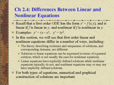
Ch 2.4: Differences Between Linear and Nonlinear Equations

1
Ch 2.4 Differences Between Linear and Nonlinear
Equations

• Recall that a first order ODE has the form y' f
  (t, y), and is linear if f is linear in y, and
  nonlinear if f is nonlinear in y.
• Examples y' t y - e t, y' t y2.
• In this section, we will see that first order
  linear and nonlinear equations differ in a number
  of ways, including
• The theory describing existence and uniqueness of
  solutions, and corresponding domains, are
  different.
• Solutions to linear equations can be expressed in
  terms of a general solution, which is not usually
  the case for nonlinear equations.
• Linear equations have explicitly defined
  solutions while nonlinear equations typically do
  not, and nonlinear equations may or may not have
  implicitly defined solutions.
• For both types of equations, numerical and
  graphical construction of solutions are important.

2
Theorem 2.4.1

• Consider the linear first order initial value
  problem
• If the functions p and g are continuous on an
  open interval (?, ? ) containing the point t
  t0, then there exists a unique solution y ?(t)
  that satisfies the IVP for each t in (?, ? ).
• Proof outline Use Ch 2.1 discussion and results

3
Theorem 2.4.2

• Consider the nonlinear first order initial value
  problem
• Suppose f and ?f/?y are continuous on some open
  rectangle (t, y) ? (?, ? ) x (?, ? ) containing
  the point (t0, y0). Then in some interval (t0 -
  h, t0 h) ? (?, ? ) there exists a unique
  solution y ?(t) that satisfies the IVP.
• Proof discussion Since there is no general
  formula for the solution of arbitrary nonlinear
  first order IVPs, this proof is difficult, and is
  beyond the scope of this course.
• It turns out that conditions stated in Thm 2.4.2
  are sufficient but not necessary to guarantee
  existence of a solution, and continuity of f
  ensures existence but not uniqueness of ?.

4
Example 1 Linear IVP

• Recall the initial value problem from Chapter 2.1
  slides
• The solution to this initial value problem is
  defined for
• t gt 0, the interval on which p(t) -2/t is
  continuous.
• If the initial condition is y(-1) 2, then the
  solution is given by same expression as above,
  but is defined on t lt 0.
• In either case, Theorem 2.4.1
• guarantees that solution is unique
• on corresponding interval.

5
Example 2 Nonlinear IVP (1 of 2)

• Consider nonlinear initial value problem from Ch
  2.2
• The functions f and ?f/?y are given by
• and are continuous except on line y 1.
• Thus we can draw an open rectangle about (0, -1)
  on which f and ?f/?y are continuous, as long as
  it doesnt cover y 1.
• How wide is rectangle? Recall solution defined
  for t gt -2, with

6
Example 2 Change Initial Condition (2 of 2)

• Our nonlinear initial value problem is
• with
• which are continuous except on line y 1.
• If we change initial condition to y(0) 1, then
  Theorem 2.4.2 is not satisfied. Solving this new
  IVP, we obtain
• Thus a solution exists but is not unique.

7
Example 3 Nonlinear IVP

• Consider nonlinear initial value problem
• The functions f and ?f/?y are given by
• Thus f continuous everywhere, but ?f/?y doesnt
  exist at y 0, and hence Theorem 2.4.2 is not
  satisfied. Solutions exist but are not unique.
  Separating variables and solving, we obtain
• If initial condition is not on t-axis, then
  Theorem 2.4.2 does guarantee existence and
  uniqueness.

8
Example 4 Nonlinear IVP

• Consider nonlinear initial value problem
• The functions f and ?f/?y are given by
• Thus f and ?f/?y are continuous at t 0, so Thm
  2.4.2 guarantees that solutions exist and are
  unique.
• Separating variables and solving, we obtain
• The solution y(t) is defined on (-?, 1). Note
  that the singularity at t 1 is not obvious from
  original IVP statement.

9
Interval of Definition Linear Equations

• By Theorem 2.4.1, the solution of a linear
  initial value problem
• exists throughout any interval about t t0 on
  which p and g are continuous.
• Vertical asymptotes or other discontinuities of
  solution can only occur at points of
  discontinuity of p or g.
• However, solution may be differentiable at points
  of discontinuity of p or g. See Chapter 2.1
  Example 3 of text.
• Compare these comments with Example 1 and with
  previous linear equations in Chapter 1 and
  Chapter 2.

10
Interval of Definition Nonlinear Equations

• In the nonlinear case, the interval on which a
  solution exists may be difficult to determine.
• The solution y ?(t) exists as long as (t,?(t))
  remains within rectangular region indicated in
  Theorem 2.4.2. This is what determines the value
  of h in that theorem. Since ?(t) is usually not
  known, it may be impossible to determine this
  region.
• In any case, the interval on which a solution
  exists may have no simple relationship to the
  function f in the differential equation y' f
  (t, y), in contrast with linear equations.
• Furthermore, any singularities in the solution
  may depend on the initial condition as well as
  the equation.
• Compare these comments to the preceding examples.

11
General Solutions

• For a first order linear equation, it is possible
  to obtain a solution containing one arbitrary
  constant, from which all solutions follow by
  specifying values for this constant.
• For nonlinear equations, such general solutions
  may not exist. That is, even though a solution
  containing an arbitrary constant may be found,
  there may be other solutions that cannot be
  obtained by specifying values for this constant.
  
• Consider Example 4 The function y 0 is a
  solution of the differential equation, but it
  cannot be obtained by specifying a value for c in
  solution found using separation of variables

12
Explicit Solutions Linear Equations

• By Theorem 2.4.1, a solution of a linear initial
  value problem
• exists throughout any interval about t t0 on
  which p and g are continuous, and this solution
  is unique.
• The solution has an explicit representation,
• and can be evaluated at any appropriate value of
  t, as long as the necessary integrals can be
  computed.

13
Explicit Solution Approximation

• For linear first order equations, an explicit
  representation for the solution can be found, as
  long as necessary integrals can be solved.
• If integrals cant be solved, then numerical
  methods are often used to approximate the
  integrals.

14
Implicit Solutions Nonlinear Equations

• For nonlinear equations, explicit representations
  of solutions may not exist.
• As we have seen, it may be possible to obtain an
  equation which implicitly defines the solution.
  If equation is simple enough, an explicit
  representation can sometimes be found.
• Otherwise, numerical calculations are necessary
  in order to determine values of y for given
  values of t. These values can then be plotted in
  a sketch of the integral curve.
• Recall the following example from
• Ch 2.2 slides

15
Direction Fields

• In addition to using numerical methods to sketch
  the integral curve, the nonlinear equation itself
  can provide enough information to sketch a
  direction field.
• The direction field can often show the
  qualitative form of solutions, and can help
  identify regions in the ty-plane where solutions
  exhibit interesting features that merit more
  detailed analytical or numerical investigations.
• Chapter 2.7 and Chapter 8 focus on numerical
  methods.