
Hidden Markov Models - PowerPoint PPT Presentation
Title: Hidden Markov Models
1
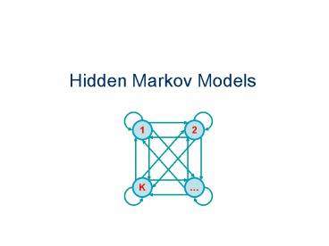
Hidden Markov Models
1
2
K
2
Outline
- Hidden Markov Models Formalism
- The Three Basic Problems of HMMs
- Solutions
- Applications of HMMs for Automatic Speech
Recognition (ASR)
3
Example The Dishonest Casino
- A casino has two dice
- Fair die
- P(1) P(2) P(3) P(5) P(6) 1/6
- Loaded die
- P(1) P(2) P(3) P(4) P(5) 1/10
- P(6) 1/2
- Casino player switches back--forth between fair
and loaded die once in a while - Game
- You bet 1
- You roll (always with a fair die)
- Casino player rolls (maybe with fair die, maybe
with loaded die) - Highest number wins 2
4
Question 1 Evaluation
- GIVEN
- A sequence of rolls by the casino player
- 12455264621461461361366616646616366163661636165
- QUESTION
- How likely is this sequence, given our model of
how the casino works? - This is the EVALUATION problem in HMMs
5
Question 2 Decoding
- GIVEN
- A sequence of rolls by the casino player
- 12455264621461461361366616646616366163661636165
- QUESTION
- What portion of the sequence was generated with
the fair die, and what portion with the loaded
die? - This is the DECODING question in HMMs
6
Question 3 Learning
- GIVEN
- A sequence of rolls by the casino player
- 12455264621461461361366616646616366163661636165
- QUESTION
- How loaded is the loaded die? How fair is the
fair die? How often does the casino player change
from fair to loaded, and back? - This is the LEARNING question in HMMs
7
The dishonest casino model
0.05
0.95
0.95
FAIR
LOADED
P(1F) 1/6 P(2F) 1/6 P(3F) 1/6 P(4F)
1/6 P(5F) 1/6 P(6F) 1/6
P(1L) 1/10 P(2L) 1/10 P(3L) 1/10 P(4L)
1/10 P(5L) 1/10 P(6L) 1/2
0.05
8
Example the dishonest casino
- Let the sequence of rolls be
- O 1, 2, 1, 5, 6, 2, 1, 6, 2, 4
- Then, what is the likelihood of
- X Fair, Fair, Fair, Fair, Fair, Fair, Fair,
Fair, Fair, Fair? - (say initial probs P(t0,Fair) ½,
P(t0,Loaded) ½) - ½ ? P(1 Fair) P(Fair Fair) P(2 Fair) P(Fair
Fair) P(4 Fair) - ½ ? (1/6)10 ? (0.95)9 .00000000521158647211
0.5 ? 10-9
9
Example the dishonest casino
- So, the likelihood the die is fair in all this
run - is just 0.521 ? 10-9
- OK, but what is the likelihood of
- X Loaded, Loaded, Loaded, Loaded, Loaded,
Loaded, Loaded, Loaded, Loaded, Loaded? - ½ ? P(1 Loaded) P(Loaded, Loaded) P(4
Loaded) - ½ ? (1/10)8 ? (1/2)2 (0.95)9 .000000000787811762
15 7.9 ? 10-10 - Therefore, it is after all 6.59 times more likely
that the die is fair all the way, than that it is
loaded all the way.
10
Example the dishonest casino
- Let the sequence of rolls be
- O 1, 6, 6, 5, 6, 2, 6, 6, 3, 6
- Now, what is the likelihood X F, F, , F?
- ½ ? (1/6)10 ? (0.95)9 0.5 ? 10-9, same as
before - What is the likelihood
- X L, L, , L?
- ½ ? (1/10)4 ? (1/2)6 (0.95)9 .000000492382351347
35 0.5 ? 10-7 - So, it is 100 times more likely the die is loaded
11
HMM Timeline
time ?
- Arrows indicate probabilistic dependencies.
- xs are hidden states, each dependent only on the
previous state. - The Markov assumption holds for the state
sequence. - os are observations, dependent only on their
corresponding hidden state.
12
HMM Formalism
- An HMM ? can be specified by 3 matrices P, A,
B - P pi are the initial state probabilities
- A aij are the state transition probabilities
Pr(xjxi) - B bik are the observation probabilities
Pr(okxi)
13
Generating a sequence by the model
- Given a HMM, we can generate a sequence of length
n as follows - Start at state xi according to prob ?i
- Emit letter o1 according to prob bi(o1)
- Go to state xj according to prob aij
- until emitting oT
1
?2
2
2
0
N
b2o1
o1
o2
o3
oT
14
The three main questions on HMMs
- Evaluation
- GIVEN a HMM ?, and a sequence O,
- FIND Prob O ?
- Decoding
- GIVEN a HMM ?, and a sequence O,
- FIND the sequence X of states that maximizes
PX O, ? - Learning
- GIVEN a sequence O,
- FIND a model ? with parameters ?, A and B
that - maximize P O ?
15
Problem 1 Evaluation
- Find the likelihood a sequence is generated by
the model
16
Probability of an Observation
o1
ot
ot-1
ot1
Given an observation sequence and a model,
compute the probability of the observation
sequence
17
Probability of an Observation
Let X x1 xt be the state sequence.
18
Probability of an Observation
19
HMM Evaluation (cont.)
- Why isnt it efficient?
- For a given state sequence of length T we have
about 2T calculations - Let N be the number of states in the graph.
- There are NT possible state sequences.
- Complexity O(2TNT )
- Can be done more efficiently by the
forward-backward (F-B) procedure.
20
The Forward Procedure (Prefix Probs)
The probability of being in state i after
generating the first t observations.
21
Forward Procedure
22
Forward Procedure
23
Forward Procedure
24
Forward Procedure
25
Forward Procedure
26
Forward Procedure
27
Forward Procedure
28
Forward Procedure
29
The Forward Procedure
- Initialization
- Iteration
- Termination
- Computational Complexity O(N2T)
30
Another Version The Backward Procedure (Suffix
Probs)
x1
xt1
xT
xt
xt-1
oT
o1
ot
ot-1
ot1
Probability of the rest of the states given the
first state
31
Problem 2 Decoding
- Find the best state sequence
32
Decoding
- Given an HMM and a new sequence of observations,
find the most probable sequence of hidden states
that generated these observations - In general, there is an exponential number of
possible sequences. - Use dynamic programming to reduce search space to
O(n2T).
33
Viterbi Algorithm
x1
xt-1
j
oT
o1
ot
ot-1
ot1
The state sequence which maximizes the
probability of seeing the observations up to time
t-1, landing in state j, and seeing the
observation at time t.
34
Viterbi Algorithm
x1
xt-1
j
oT
o1
ot
ot-1
ot1
Initialization
35
Viterbi Algorithm
x1
xt-1
xt
xt1
Recursion
Prob. of ML state
Name of ML state
36
Viterbi Algorithm
x1
xt-1
xt
xt1
xT
Termination
Read out the most likely state sequence,
working backwards.
37
Problem 3 Learning
- Re-estimate the parameters of the model based on
training data
38
Learning by Parameter Estimation
- Goal Given an observation sequence, find the
model that is most likely to produce that
sequence. - Problem We dont know the relative frequencies
of hidden visited states. - No analytical solution is known for HMMs.
- We will approach the solution by successive
approximations.
39
The Baum-Welch Algorithm
- Find the expected frequencies of possible values
of the hidden variables. - Compute the maximum likelihood distributions of
the hidden variables (by normalizing, as usual
for MLE). - Repeat until convergence.
- This is the Expectation-Maximization (EM)
algorithm for parameter estimation. - Applicable to any stochastic process, in theory.
- Special case for HMMs is called the Baum-Welch
algorithm.
40
Arc and State Probabilities
A
A
A
A
B
B
B
B
B
Probability of traversing an arc From state i (at
time t) to state j (at time t1)
Probability of being in state i at time t.
41
Aggregation and Normalization
A
A
A
A
B
B
B
B
B
Now we can compute the new MLEs of the model
parameters.
42
The Baum-Welch Algorithm
- Initialize A,B and ? (Pick the best-guess for
model parameters or arbitrary) - Repeat
- Calculate and
- Calculate and
- Estimate , and
- Until the changes are small enough
43
The Baum-Welch Algorithm Comments
- Time Complexity
- iterations ? O(N2T)
- Guaranteed to increase the (log) likelihood of
the model - P(? O) P(O, ?) / P(O) P(O ?) / ( P(O)
P(?) ) - Not guaranteed to find globally best parameters
- Converges to local optimum, depending on initial
conditions - Too many parameters / too large model -
Overtraining
44
Application Automatic Speech Recognition
45
Examples (1)
46
Examples (2)
47
Examples (3)
48
Examples (4)
49
(No Transcript)
50
Phones
51
Speech Signal
- Waveform
- Spectrogram
52
Speech Signal cont.
Articulation
53
Feature Extraction
Frame 1
Frame 2
Feature VectorX1
Feature VectorX2
54
(No Transcript)
55
(No Transcript)
Recommended
CrystalGraphics Presentations


