Linear Regression

1
Linear Regression

• Hypothesis testing and Estimation

2

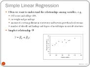
• Assume that we have collected data on two
  variables X and Y. Let
• (x1, y1) (x2, y2) (x3, y3) (xn, yn)
• denote the pairs of measurements on the on two
  variables X and Y for n cases in a sample (or
  population)

3
The Statistical Model
4

• Each yi is assumed to be randomly generated from
  a normal distribution with
• mean mi a bxi and
• standard deviation s.
• (a, b and s are unknown)

5
The Data The Linear Regression Model

• The data falls roughly about a straight line.

unseen
6
The Least Squares Line

• Fitting the best straight line
• to linear data

7

• Let
• Y a b X
• denote an arbitrary equation of a straight line.
• a and b are known values.
• This equation can be used to predict for each
  value of X, the value of Y.
• For example, if X xi (as for the ith case) then
  the predicted value of Y is

8

• The residual
• can be computed for each case in the sample,
• The residual sum of squares (RSS) is
• a measure of the goodness of fit of the line
• Y a bX to the data

9

• The optimal choice of a and b will result in the
  residual sum of squares
• attaining a minimum.
• If this is the case than the line
• Y a bX
• is called the Least Squares Line

10

• The equation for the least squares line
• Let

11
Computing Formulae

12

• Then the slope of the least squares line can be
  shown to be

13

• and the intercept of the least squares line can
  be shown to be

14

• The residual sum of Squares

15

• Estimating s, the standard deviation in the
  regression model

This estimate of s is said to be based on n 2
degrees of freedom
16
Sampling distributions of the estimators
17

• The sampling distribution slope of the least
  squares line

It can be shown that b has a normal distribution
with mean and standard deviation
18

• Thus

has a standard normal distribution, and
has a t distribution with df n - 2
19

• (1 a)100 Confidence Limits for slope b

ta/2 critical value for the t-distribution with n
2 degrees of freedom
20

• Testing the slope

The test statistic is
- has a t distribution with df n 2 if H0 is
true.
21

• The Critical Region

Reject
df n 2
This is a two tailed tests. One tailed tests are
also possible
22

• The sampling distribution intercept of the least
  squares line

It can be shown that a has a normal distribution
with mean and standard deviation
23

• Thus

has a standard normal distribution and
has a t distribution with df n - 2
24

• (1 a)100 Confidence Limits for intercept a

ta/2 critical value for the t-distribution with n
2 degrees of freedom
25

• Testing the intercept

The test statistic is
- has a t distribution with df n 2 if H0 is
true.
26

• The Critical Region

Reject
df n 2
27
Example
28
The following data showed the per capita
consumption of cigarettes per month (X) in
various countries in 1930, and the death rates
from lung cancer for men in 1950. TABLE Per
capita consumption of cigarettes per month (Xi)
in n 11 countries in 1930, and the death
rates, Yi (per 100,000), from lung cancer for men
in 1950.  Country (i) Xi Yi Australia 48 18
Canada 50 15 Denmark 38 17 Finland 110 35 Great
Britain 110 46 Holland 49 24 Iceland 23 6 Norw
ay 25 9 Sweden 30 11 Switzerland 51 25 USA 130
20 
29
(No Transcript)
30
Fitting the Least Squares Line

31
Fitting the Least Squares Line

First compute the following three quantities
32
Computing Estimate of Slope (b), Intercept (a)
and standard deviation (s),
33

• 95 Confidence Limits for slope b

0.0706 to 0.3862
t.025 2.262 critical value for the
t-distribution with 9 degrees of freedom
34

• 95 Confidence Limits for intercept a

-4.34 to 17.85
t.025 2.262 critical value for the
t-distribution with 9 degrees of freedom
35
95 confidence Limits for slope 0.0706 to 0.3862
95 confidence Limits for intercept -4.34 to 17.85
36

• Testing the positive slope

The test statistic is
37

• The Critical Region

Reject
df 11 2 9
A one tailed test
38
we reject
and conclude
39
Confidence Limits for Points on the Regression
Line

• The intercept a is a specific point on the
  regression line.
• It is the y coordinate of the point on the
  regression line when x 0.
• It is the predicted value of y when x 0.
• We may also be interested in other points on the
  regression line. e.g. when x x0
• In this case the y coordinate of the point on
  the regression line when x x0 is a b x0

40
x0
41

• (1- a)100 Confidence Limits for a b x0

ta/2 is the a/2 critical value for the
t-distribution with n - 2 degrees of freedom
42
Prediction Limits for new values of the Dependent
variable y

• An important application of the regression line
  is prediction.
• Knowing the value of x (x0) what is the value of
  y?
• The predicted value of y when x x0 is
• This in turn can be estimated by.

43

• The predictor
• Gives only a single value for y.
• A more appropriate piece of information would be
  a range of values.
• A range of values that has a fixed probability of
  capturing the value for y.
• A (1- a)100 prediction interval for y.

44

• (1- a)100 Prediction Limits for y when x x0

ta/2 is the a/2 critical value for the
t-distribution with n - 2 degrees of freedom
45
Example

• In this example we are studying building fires in
  a city and interested in the relationship
  between

1. X the distance of the closest fire hall and
   the building that puts out the alarm

and

1. Y cost of the damage (1000)

The data was collected on n 15 fires.
46
The Data
47
Scatter Plot
48
Computations
49
Computations Continued
50
Computations Continued
51
Computations Continued
52

• 95 Confidence Limits for slope b

4.07 to 5.77
t.025 2.160 critical value for the
t-distribution with 13 degrees of freedom
53

• 95 Confidence Limits for intercept a

7.21 to 13.35
t.025 2.160 critical value for the
t-distribution with 13 degrees of freedom
54
Least Squares Line
55

• (1- a)100 Confidence Limits for a b x0

ta/2 is the a/2 critical value for the
t-distribution with n - 2 degrees of freedom
56
95 Confidence Limits for a b x0
57
95 Confidence Limits for a b x0
58

• (1- a)100 Prediction Limits for y when x x0

ta/2 is the a/2 critical value for the
t-distribution with n - 2 degrees of freedom
59
95 Prediction Limits for y when x x0
60
95 Prediction Limits for y when x x0
61
Linear RegressionSummary

• Hypothesis testing and Estimation

62

• (1 a)100 Confidence Limits for slope b

ta/2 critical value for the t-distribution with n
2 degrees of freedom
63

• Testing the slope

The test statistic is
- has a t distribution with df n 2 if H0 is
true.
64

• (1 a)100 Confidence Limits for intercept a

ta/2 critical value for the t-distribution with n
2 degrees of freedom
65

• Testing the intercept

The test statistic is
- has a t distribution with df n 2 if H0 is
true.
66

• (1- a)100 Confidence Limits for a b x0

ta/2 is the a/2 critical value for the
t-distribution with n - 2 degrees of freedom
67

• (1- a)100 Prediction Limits for y when x x0

ta/2 is the a/2 critical value for the
t-distribution with n - 2 degrees of freedom
68
Correlation
69
Definition
The statistic
is called Pearsons correlation coefficient
70
Properties

• -1 r 1, r 1, r2 1
• r 1 (r 1 or -1) if the points
• (x1, y1), (x2, y2), , (xn, yn) lie along a
  straight line. (positive slope for 1, negative
  slope for -1)

71
The test for independence (zero correlation)
H0 X and Y are independent HA X and Y are
correlated
The test statistic
The Critical region
Reject H0 if t gt ta/2 (df n 2)
This is a two-tailed critical region, the
critical region could also be one-tailed
72
Example

• In this example we are studying building fires in
  a city and interested in the relationship
  between

1. X the distance of the closest fire hall and
   the building that puts out the alarm

and

1. Y cost of the damage (1000)

The data was collected on n 15 fires.
73
The Data
74
Scatter Plot
75
Computations
76
Computations Continued
77
Computations Continued
78
The correlation coefficient
The test for independence (zero correlation)
The test statistic
We reject H0 independence, if t gt t0.025
2.160
H0 independence, is rejected
79
Relationship between Regression and Correlation
80
Recall
Also
since
Thus the slope of the least squares line is
simply the ratio of the standard deviations the
correlation coefficient
81
The test for independence (zero correlation)
H0 X and Y are independent HA X and Y are
correlated
Uses the test statistic
Note
and
82
The two tests

1. The test for independence (zero correlation)

H0 X and Y are independent HA X and Y are
correlated

1. The test for zero slope

H0 b 0. HA b ? 0
are equivalent
83

1. the test statistic for independence

84
Regression (in general)
85

• In many experiments we would have collected data
  on a single variable Y (the dependent variable )
  and on p (say) other variables X1, X2, X3, ... ,
  Xp (the independent variables).
•  
• One is interested in determining a model that
  describes the relationship between Y (the
  response (dependent) variable) and X1, X2, , Xp
  (the predictor (independent) variables.
• This model can be used for
• Prediction
• Controlling Y by manipulating X1, X2, , Xp
•  

86

•  
• The Model
• is an equation of the form
• Y f(X1, X2,... ,Xp q1, q2, ... , qq) e
• where q1, q2, ... , qq are unknown parameters of
  the function f and e is a random disturbance
  (usually assumed to have a normal distribution
  with mean 0 and standard deviation s).

87

• Examples
• Y Blood Pressure, X age
• The model
• Y a bX e,thus q1 a and q2 b.
• This model is called
• the simple Linear Regression Model

88

• Y average of five best times for running the
  100m, X the year
• The model
• Y a e-bX g e, thus q1 a, q2 b and q2
  g.
• This model is called
• the exponential Regression Model

Y a e-bX g
89

• Y gas mileage ( mpg) of a car brand
• X1 engine size
• X2 horsepower
• X3 weight
• The model
• Y b0 b1 X1 b2 X2 b3 X3 e.
• This model is called
• the Multiple Linear Regression Model

90
The Multiple Linear Regression Model
91

• In Multiple Linear Regression we assume the
  following model
•  
• Y b0 b1 X1 b2 X2 ... bp Xp e
•  
• This model is called the Multiple Linear
  Regression Model.
• Again are unknown parameters of the model and
  where b0, b1, b2, ... , bp are unknown
  parameters and e is a random disturbance assumed
  to have a normal distribution with mean 0 and
  standard deviation s.

92
The importance of the Linear model

• 1.     It is the simplest form of a model in
  which each dependent variable has some effect on
  the independent variable Y.
• When fitting models to data one tries to find the
  simplest form of a model that still adequately
  describes the relationship between the dependent
  variable and the independent variables.
• The linear model is sometimes the first model to
  be fitted and only abandoned if it turns out to
  be inadequate.

93

• In many instance a linear model is the most
  appropriate model to describe the dependence
  relationship between the dependent variable and
  the independent variables.
• This will be true if the dependent variable
  increases at a constant rate as any or the
  independent variables is increased while holding
  the other independent variables constant.

94

• 3.     Many non-Linear models can be Linearized
  (put into the form of a Linear model by
  appropriately transformation the dependent
  variables and/or any or all of the independent
  variables.)
• This important fact ensures the wide utility of
  the Linear model. (i.e. the fact the many
  non-linear models are linearizable.)

95
An Example

• The following data comes from an experiment that
  was interested in investigating the source from
  which corn plants in various soils obtain their
  phosphorous.
• The concentration of inorganic phosphorous (X1)
  and the concentration of organic phosphorous (X2)
  was measured in the soil of n 18 test plots.
• In addition the phosphorous content (Y) of corn
  grown in the soil was also measured. The data is
  displayed below

96


97
Equation Y 56.2510241 1.78977412 X1
0.08664925 X2
98
(No Transcript)
99
The Multiple Linear Regression Model
100

• In Multiple Linear Regression we assume the
  following model
•  
• Y b0 b1 X1 b2 X2 ... bp Xp e
•  
• This model is called the Multiple Linear
  Regression Model.
• Again are unknown parameters of the model and
  where b0, b1, b2, ... , bp are unknown
  parameters and e is a random disturbance assumed
  to have a normal distribution with mean 0 and
  standard deviation s.

101
Summary of the Statistics used in Multiple
Regression
102

• The Least Squares Estimates

- the values that minimize
103

• The Analysis of Variance Table Entries
• a) Adjusted Total Sum of Squares (SSTotal)
• b) Residual Sum of Squares (SSError)
• c) Regression Sum of Squares (SSReg)
• Note
• i.e. SSTotal SSReg SSError
•  

104
The Analysis of Variance Table

• Source Sum of Squares d.f. Mean Square F
• Regression SSReg p SSReg/p MSReg MSReg/s2
• Error SSError n-p-1 SSError/(n-p-1) MSError
  s2
• Total SSTotal n-1

105
Uses

• 1. To estimate s2 (the error variance).
• - Use s2 MSError to estimate s2.
• To test the Hypothesis
• H0 b1 b2 ... bp 0.
• Use the test statistic

- Reject H0 if F gt Fa(p,n-p-1).
106

• 3. To compute other statistics that are useful in
  describing the relationship between Y (the
  dependent variable) and X1, X2, ... ,Xp (the
  independent variables).
• a) R2 the coefficient of determination
• SSReg/SSTotal
• the proportion of variance in Y explained by
• X1, X2, ... ,Xp
• 1 - R2 the proportion of variance in Y
• that is left unexplained by X1, X2, ... , Xp
• SSError/SSTotal.

107

• b) Ra2 "R2 adjusted" for degrees of freedom.
• 1 -the proportion of variance in Y that is
  left
• unexplained by X1, X2,... , Xp adjusted
  for d.f.

108

• c) R ÖR2 the Multiple correlation
  coefficient of Y with X1, X2, ... ,Xp
• the maximum correlation between Y and a
  linear combination of X1, X2, ... ,Xp
• Comment The statistics F, R2, Ra2 and R are
  equivalent statistics.

109
Using Statistical Packages

• To perform Multiple Regression

110
Using SPSS
Note The use of another statistical package such
as Minitab is similar to using SPSS
111
After starting the SSPS program the following
dialogue box appears
112
If you select Opening an existing file and press
OK the following dialogue box appears
113
The following dialogue box appears
114
If the variable names are in the file ask it to
read the names. If you do not specify the Range
the program will identify the Range
Once you click OK, two windows will appear
115
One that will contain the output
116
The other containing the data
117
To perform any statistical Analysis select the
Analyze menu
118
Then select Regression and Linear.
119
The following Regression dialogue box appears
120
Select the Dependent variable Y.
121
Select the Independent variables X1, X2, etc.
122
If you select the Method - Enter.
123

• All variables will be put into the equation.

There are also several other methods that can be
used

1. Forward selection
2. Backward Elimination
3. Stepwise Regression

124
(No Transcript)
125

• Forward selection

1. This method starts with no variables in the
   equation
2. Carries out statistical tests on variables not in
   the equation to see which have a significant
   effect on the dependent variable.
3. Adds the most significant.
4. Continues until all variables not in the equation
   have no significant effect on the dependent
   variable.

126

• Backward Elimination

1. This method starts with all variables in the
   equation
2. Carries out statistical tests on variables in the
   equation to see which have no significant effect
   on the dependent variable.
3. Deletes the least significant.
4. Continues until all variables in the equation
   have a significant effect on the dependent
   variable.

127

• Stepwise Regression (uses both forward and
  backward techniques)

1. This method starts with no variables in the
   equation
2. Carries out statistical tests on variables not in
   the equation to see which have a significant
   effect on the dependent variable.
3. It then adds the most significant.
4. After a variable is added it checks to see if any
   variables added earlier can now be deleted.
5. Continues until all variables not in the equation
   have no significant effect on the dependent
   variable.

128

• All of these methods are procedures for
  attempting to find the best equation

The best equation is the equation that is the
simplest (not containing variables that are not
important) yet adequate (containing variables
that are important)
129
Once the dependent variable, the independent
variables and the Method have been selected if
you press OK, the Analysis will be performed.
130
The output will contain the following table
R2 and R2 adjusted measures the proportion of
variance in Y that is explained by X1, X2, X3,
etc (67.6 and 67.3)
R is the Multiple correlation coefficient (the
maximum correlation between Y and a linear
combination of X1, X2, X3, etc)
131
The next table is the Analysis of Variance Table
The F test is testing if the regression
coefficients of the predictor variables are all
zero. Namely none of the independent variables
X1, X2, X3, etc have any effect on Y
132
The final table in the output
Gives the estimates of the regression
coefficients, there standard error and the t test
for testing if they are zeroNote Engine size
has no significant effect on Mileage
133
The estimated equation from the table below
Is
134
Note the equation is
Mileage decreases with

1. With increases in Engine Size (not significant, p
   0.432)With increases in Horsepower
   (significant, p 0.000)With increases in Weight
   (significant, p 0.000)

135
The Multiple Linear Regression ModelSummary
136

• In many experiments we would have collected data
  on a single variable Y (the dependent variable )
  and on p (say) other variables X1, X2, X3, ... ,
  Xp (the independent variables).
•  
• One is interested in determining a model that
  describes the relationship between Y (the
  response (dependent) variable) and X1, X2, , Xp
  (the predictor (independent) variables.
• This model can be used for
• Prediction
• Controlling Y by manipulating X1, X2, , Xp
•  

137

• In Multiple Linear Regression we assume the
  following model
•  
• Y b0 b1 X1 b2 X2 ... bp Xp e
•  
• This model is called the Multiple Linear
  Regression Model.
• Again are unknown parameters of the model and
  where b0, b1, b2, ... , bp are unknown
  parameters and e is a random disturbance assumed
  to have a normal distribution with mean 0 and
  standard deviation s.

138
The Statistics in Multiple Regression
139

• The Least Squares Estimates

- the values that minimize
140

• The Analysis of Variance Table Entries
• a) Adjusted Total Sum of Squares (SSTotal)
• b) Residual Sum of Squares (SSError)
• c) Regression Sum of Squares (SSReg)
• Note
• i.e. SSTotal SSReg SSError
•  

141
The Analysis of Variance Table

• Source Sum of Squares d.f. Mean Square F
• Regression SSReg p SSReg/p MSReg MSReg/s2
• Error SSError n-p-1 SSError/(n-p-1) MSError
  s2
• Total SSTotal n-1

142

• Important Summary Statistics
• a) R2 the coefficient of determination
• SSReg/SSTotal
• the proportion of variance in Y explained by
• X1, X2, ... ,Xp
• 1 - R2 the proportion of variance in Y
• that is left unexplained by X1, X2, ... , Xp
• SSError/SSTotal.

143

• b) Ra2 "R2 adjusted" for degrees of freedom.
• 1 -the proportion of variance in Y that is
  left
• unexplained by X1, X2,... , Xp adjusted
  for d.f.

144

• c) R ÖR2 the Multiple correlation
  coefficient of Y with X1, X2, ... ,Xp
• the maximum correlation between Y and a
  linear combination of X1, X2, ... ,Xp

145
Example

• In this example we are interested in how
• Y mileage (mpg)
• depends on
• X1 engine size
• X2 vehicle weight
• X3 engine horse power

146
The output from SPSS
R2 and R2 adjusted measures the proportion of
variance in Y that is explained by X1, X2, X3,
etc (67.6 and 67.3)
R is the Multiple correlation coefficient (the
maximum correlation between Y and a linear
combination of X1, X2, X3, etc)
147
The next table is the Analysis of Variance Table
The F test is testing if the regression
coefficients of the predictor variables are all
zero. Namely none of the independent variables
X1, X2, X3, etc have any effect on Y
148
The final table in the output
Gives the estimates of the regression
coefficients, there standard error and the t test
for testing if they are zeroNote Engine size
has no significant effect on Mileage
149
The estimated equation from the table below
Is
150
Note the equation is
Mileage decreases with

1. With increases in Engine Size (not significant, p
   0.432)With increases in Horsepower
   (significant, p 0.000)With increases in Weight
   (significant, p 0.000)

151
Logistic regression
152

• Recall the simple linear regression model
• y b0 b1x e

where we are trying to predict a continuous
dependent variable y from a continuous
independent variable x.
This model can be extended to Multiple linear
regression model y b0 b1x1 b2x2
bpxp e
Here we are trying to predict a continuous
dependent variable y from a several continuous
dependent variables x1 , x2 , , xp .
153
Now suppose the dependent variable y is binary.
It takes on two values Success (1) or
Failure (0)
We are interested in predicting a y from a
continuous dependent variable x.
This is the situation in which Logistic
Regression is used
154
Example

• We are interested how the success (y) of a new
  antibiotic cream is curing acne problems and
  how it depends on the amount (x) that is applied
  daily.
• The values of y are 1 (Success) or 0 (Failure).
• The values of x range over a continuum

155
The logisitic Regression Model

• Let p denote Py 1 PSuccess.
• This quantity will increase with the value of x.

is called the odds ratio
The ratio
This quantity will also increase with the value
of x, ranging from zero to infinity.
The quantity
is called the log odds ratio
156
Example odds ratio, log odds ratio

• Suppose a die is rolled
• Success roll a six, p 1/6

The odds ratio
The log odds ratio
157
The logisitic Regression Model
Assumes the log odds ratio is linearly related to
x.
i. e.
In terms of the odds ratio
158
The logisitic Regression Model
Solving for p in terms x.
or
159
Interpretation of the parameter b0 (determines
the intercept)
p
x
160
Interpretation of the parameter b1 (determines
when p is 0.50 (along with b0))
p
when
x
161
Also
when
is the rate of increase in p with respect to x
when p 0.50
162
Interpretation of the parameter b1 (determines
slope when p is 0.50 )
p
x
163
The data

• The data will for each case consist of

1. a value for x, the continuous independent
   variable
2. a value for y (1 or 0) (Success or Failure)

Total of n 250 cases
164
(No Transcript)
165
Estimation of the parameters

• The parameters are estimated by Maximum
  Likelihood estimation and require a statistical
  package such as SPSS

166
Using SPSS to perform Logistic regression

• Open the data file

167

• Choose from the menu
• Analyze -gt Regression -gt Binary Logistic

168

• The following dialogue box appears

Select the dependent variable (y) and the
independent variable (x) (covariate). Press OK.
169

• Here is the output

The Estimates and their S.E.
170
The parameter Estimates
171
Interpretation of the parameter b0 (determines
the intercept)
Interpretation of the parameter b1 (determines
when p is 0.50 (along with b0))
172
Another interpretation of the parameter b1
is the rate of increase in p with respect to x
when p 0.50
173
The Logistic Regression Model
The dependent variable y is binary. It takes on
two values Success (1) or Failure (0)
We are interested in predicting a y from a
continuous dependent variable x.
174
The logisitic Regression Model

• Let p denote Py 1 PSuccess.
• This quantity will increase with the value of x.

is called the odds ratio
The ratio
This quantity will also increase with the value
of x, ranging from zero to infinity.
The quantity
is called the log odds ratio
175
The logisitic Regression Model
Assumes the log odds ratio is linearly related to
x.
i. e.
In terms of the odds ratio
176
The logisitic Regression Model
In terms of p
177
The graph of p vs x
p
x
178
The Multiple Logistic Regression model
179

• Here we attempt to predict the outcome of a
  binary response variable Y from several
  independent variables X1, X2 , etc

180
Multiple Logistic Regression an example

• In this example we are interested in determining
  the risk of infants (who were born prematurely)
  of developing BPD (bronchopulmonary dysplasia)
• More specifically we are interested in developing
  a predictive model which will determine the
  probability of developing BPD from
• X1 gestational Age and X2 Birthweight

181

• For n 223 infants in prenatal ward the
  following measurements were determined

1. X1 gestational Age (weeks),
2. X2 Birth weight (grams) and
3. Y presence of BPD

182
The data
183
The results
184
Graph Showing Risk of BPD vs GA and BrthWt
185
Non-Parametric Statistics