Aggregate Supply

1
Aggregate Supply Aggregate Demand
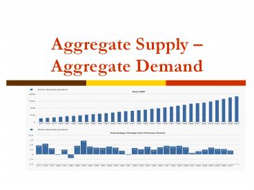
2
GDP 2007 to 2010
3
What is Aggregate Demand?

• A schedule or curve showing amounts of real
  output that buyers collectively desire to
  purchase at each possible price level.
• Think Why does AD slope downward?

4
Think Why does AD slope downward?
Vertical axis represents Price level for ALL
final goods And services
The aggregate price level Is measured by either
GDP Deflator or CPI
Price level
The horizontal axis represents the real quantity
of all GS purchased as measured by the level of
REAL GDP
AD
Real domestic output, GDP
Inverse Relationship
5
Vertical and Horizontal Axis
Horizontal axis GDP Vertical axis GDP
deflator (includes CIG) or CPI. Government
uses the deflator so it get a lower number.
A broader measure of price level includes
airplanes, dentist Visits, pizzas, new shopping
centers, etc.
6

• ASSUMPTION for Aggregate demand IS If Price
  level is decreasing, so are incomes.

Economy moves down its AD curve Moves to lower
price level remember circular flow model- (when
consumers pay lower prices for goods and
services Less nominal income flows to
resource suppliers .
7

• There are 3 Reasons that cause the Aggregate
• Demand Curve to be downward sloping.
• Real Balance Effect (Wealth effect)
• Interest Rate Effect
• International Trade Effect

8
Real Balance Effect

• Price level falls- causes purchasing power to
  rise translates into more money to spend or
  monetary wealth improves.
• Real Balance Effect (or wealth effect) Higher
  price level means less consumption spending.

9
Real Balance EffectHigher price level reduces
real value of purchasing power of publics
accumulated savings
The change in the purchasing power of
dollar- Relates to assets that result from a
change in the price level
10
Interest Rate Effect

• Inverse relationship between price level and
  quantity demanded of GDP because households and
  businesses adjust to interest rates for those
  interest-sensitive purchases.
• Price level falls (bundle of goods costs less)
  rest of money into savings, more money available
  for borrowing interest rate down.
• Think of money as stationary demand drives up
  price of money.

11
Interest Rate continued

• Now if bundle of goods increases want to
  purchase interest sensitive good, cost to borrow
  is up.
• An increase in money demand will drive up the
  price paid for its use
• use of money interest rate
• As price level rises, houses and firms require
  more money to handle transactions

12
International Trade Effect (Open Economy Effect)

• FYI An open economy is global, a closed economy
  is domestic.
• The Open Economy Effect
• Higher price levels result in foreigners
  desiring to buy fewer American-made goods while
  Americans desire more foreign-made goods (i.e.,
  net exports fall).
• Equivalent to a reduction in the amount of real
  goods and services purchased in the U.S.
• When Demand for exports decreases, this is an
  unfavorable balance of trade (imports exceed
  exports)

13
Macro AD vs Micro D

• Aggregate Demand versus Demand for a Single Good
• When the aggregate demand curve is derived, we
  are looking at the entire circular flow of income
  and product.(if AD moves to lower general price
  level- circular flow tells us when consumers pay
  lower prices less nominal income flows to
  resource suppliers

14
Demand for Single good (deals with income effect
and substitution effect

• When a market demand curve is derived, we are
  looking at a single product in one market only.
• (i.e. income effect and substitution effect)
• If prices go down for cars, have more income to
  spend someplace else.
• If price of certain items go up, we can
  substitute in many cases.

15
Change in QAD and Change in AD

• What is the difference?

PL
PL
A
B
AD 2
AD1
GDP
GDP
16
Difference between Quantity of AD and Change of AD

• QAD movement up or down as result of price
  level changing (ONLY)
• Change in AD
• Change in any of the component parts of AD (C
  I G Net Exports)

17
DETERMINANTS OF AGGREGATE DEMAND
Change in Consumer Spending

• Consumer Wealth
• Consumer Expectations (expect higher prices)
• Interest rate (interest sensitive durables)
• Taxes
• Think in aggregate terms

18
Changes in Investment Spending

• Real Interest Rates (rates high- not much I
  taking place)
• Expected Future Sales (health of economy-
  confidence is big)
• Business Taxes (higher taxes less profit)

19
Government Spending

• This will be discussed further, but anytime
  government spends, it has an affect on GDP.
• Infrastructure Health CareSupplies for
  military
• Education
• Etc.

20

• Net Export Spending
• National Income Abroad-(when foreign nations do
  well, their incomes are higher- can buy more U.S.
  goods and services. U.S. exports rise)
• Exchange Rates- Price of one nations currency in
  terms of another. Dollar vs Euro
• Our currency appreciates if it takes more foreign
  to buy it.. (depreciates if it takes more of
  ours to buy theirs.) 1.00 to 1.25 Euro.
• Depreciation of nations currency makes foreign
  goods more expensive (but attracts foreigners to
  buy our goods.) Our exports rise. this is why
  the Fed has not worried about our low dollar
  valuation.

21
Factors That Change Aggregate Demand
Consumption/Interest Rates
Interest Rate ? ? C? ? AD?
Interest Rate ? ? C ? ? AD?
22
Factors That Change Aggregate Demand
Investment/ Interest Rates
Interest rates ? ? I? ? AD?
Interest rates ? ? I ? ? AD?
23
Factors That Change Aggregate Demand
Investment/ Business Taxes
Business taxes? ? I? ? AD?
Business taxes? ? I? ? AD?
24
Long-Run Equilibrium and the Price Level

• For the economy as a whole, long-run equilibrium
  occurs at the price level where the aggregate
  demand curve (AD) crosses the long-run aggregate
  supply curve (LRAS).

25
Figure 10-5 Long-Run Economywide Equilibrium
26
OK One more time..

• Component parts of GDP?
• C I G (X-M) GDP
• Long-Run Aggregate Supply Curve (LRAS)
• A vertical line representing the real output of
  goods and services after full adjustment has
  occurred
• It represents the real GDP of the economy under
  conditions of full employment the economy is on
  its production possibilities curve

27
The Production Possibilities and the Economys
Long-Run Aggregate Supply Curve
28
Output Growth and the Long-Run Aggregate Supply
Curve (cont'd)

• LRAS is vertical
• Input prices fully adjust to changes in output
  prices
• Suppliers have no incentive to increase output
• Unemployment is at the natural rate
• Determined by endowments and technology (or
  existing resources)

29
Output Growth and the Long-Run Aggregate Supply
Curve (cont'd)

• Growth is shown by outward shifts of either the
  production possibilities curve or the LRAS curve
  caused by
• Growth of population and the labor-force
  participation rate
• Capital accumulation
• Improvements in technology

30
What does Long Run Equilibrium Mean?

• Economy is a full employment
• Any additional production would be difficult to
  achieve.
• Economy operating at natural rate of unemployment
  (anyone wanting jobhave it.)
• Equate the LRAS curve with bowed line on PPC.
• To extend either would be to discover new
  resources RD

31
Full Employment

• The condition that exists when the
  unemployment rate is equal to the natural
  unemployment rate.
• Full productive capacity has been
• Reached.

32
Image Cylinder Economy
Businesses, factories, economynot working at
full capacity
33
Full Employment
AD
AS
LRAS
34
SRAS (short run aggregate supply)

• Period where adjustment occurs.
• Direct relationship
• As the output increases that puts upward pressure
  on price.
• Movement on the curve denotes the relationship
  between price level and real output.

35
SRAS.Shift

• Shift in the curve denotes determinates that
  affect more or less real output production at
  various price levels.
• Determinants
• Change in input prices (steel, plastic, wool
  change in resource availability )
• Change in productivity ( Shift right -
  Shift left) (more for less is the object)
• Change in legal environment (contracts, taxes,
  subsidies)

36
AD and SRAS
37

• LRAS long-run aggregate supply
• LRAS is a vertical line reflecting that LR
  Aggregate Supply is not affected by changes in
  PL.
• The LRAS is labeled as the natural level of real
  GDP
• The natural level of real GDP is defined as the
  level of real GDP that arises when the economy is
  fully employing all of its available input
  resources ( We are in agreement that it hovers
  around 5)

38
Long Run Aggregate Supply
P
LRASLR
Price level
Long-run Aggregate Supply
Full-Employment
Q
Qf
Real domestic output, GDP
39
Real Rate Of Interest
D2
D1
Money Supply
Can a Change in Money Supply Change AD? Probably
but it is a chain of events.MS changes, then
Interest Rates, then chance in consumption and
investment. Then Change in AD
40
Equilibrium States of the Economy
During the time an economy moves from one
equilibrium to another, it is said to be in
disequilibrium.
41
Unanticipated Increase in Aggregate Demand

• In response to an unanticipated increase in AD
  for goods services (shift from AD1 to AD2),
  prices will rise to P105 and output will
  temporarily exceed full-employment capacity
  (increases to Y2).

42
Growth in Aggregate Supply

• Here we illustrate the impact of economic growth
  due to capital formation or a technological
  advancement, for example.

• Both LRAS and SRAS increase (to LRAS2 and SRAS2)
  the full employment output of the economy expands
  from YF1 to YF2.

• A sustainable, higher level of real output and
  real income is the result. If the money
  supply is held constant, a new long-run
  equilibrium will emerge at a larger output rate
  (YF2) and lower price level (P2).

43
Effects of Adverse Supply Shock

• The higher resource prices shift the SRAS curve
  to the left in the short-run, the price level
  rises to P110 and output falls to Y2.

• What happens in the long-run depends on whether
  the reduction in the supply of resources is
  temporary or permanent.

• If temporary, resource prices fall in the future,
  permitting the economy to return to its original
  equilibrium (A).

• If permanent, the productive potential of the
  economy will shrink (LRAS shifts to the left) and
  (B) will become the long-run equilibrium.

44
INCREASES IN AD DEMAND-PULL INFLATION
P
AS
AD1
AD2
P2
Price Level
P1
Q
Q1
Q2
Qf
Real Domestic Output, GDP
45
DECREASES IN AS COST-PUSH INFLATION
AS2
P
AS1
b
P2
Price Level
a
P1
AD1
Q
Q1
Qf
Real Domestic Output, GDP
46
(No Transcript)
47

• Non-governmental actions that shift AS
• Shift AS left
• Raw materials cost rise
• Wages rise faster than productivity
• Worker productivity decreases
• Obsolescence
• Wars
• Natural disasters

48
Fiscal Policy

• Governmental actions that shift AD
• Shift AD right
• Govt spending increases
• Taxes decreases
• Money Supply increases
• Shift AD left
• G decreases
• T increases
• MS decreases

49
KILEY SAYS THAT'S ALL!