What is it

1
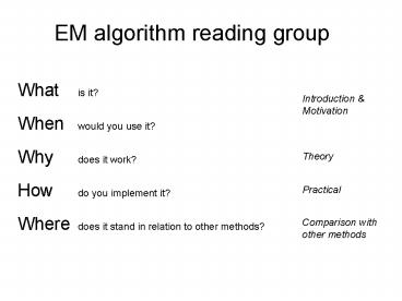
EM algorithm reading group
What is it? When would you use it? Why does
it work? How do you implement it? Where does
it stand in relation to other methods?
Introduction Motivation
Theory
Practical
Comparison with other methods
2
Expectation Maximization (EM)

• Iterative method for parameter estimation where
  you have missing data
• Has two steps Expectation (E) and Maximization
  (M)
• Applicable to a wide range of problems
• Old idea (late 50s) but formalized by Dempster,
  Laird and Rubin in 1977
• Subject of much investigation. See McLachlan
  Krishnan book 1997.

3
Applications of EM (1)

• Fitting mixture models

4
Applications of EM (2)

• Probabilistic Latent Semantic Analysis (pLSA)
• Technique from text community

P(wz)
P(zd)
P(w,d)
Z
W
W
D
Z
D
5
Applications of EM (3)

• Learning parts and structure models

6
Applications of EM (4)

• Automatic segmentation of layers in video

http//www.psi.toronto.edu/images/figures/cutouts_
vid.gif
7
Motivating example
Data
OBJECTIVE Fit mixture of Gaussian model with C2
components
Model
where
P(x?)
Parameters
keep
fixed
i.e. only estimate
x
8
Likelihood function
Likelihood is a function of parameters,
?Probability is a function of r.v. x
DIFFERENT TO LAST PLOT
9
Probabilistic model
Imagine model generating data Need to introduce
label, z, for each data point Label is called a
latent variable also called hidden, unobserved,
missing
0
1
-2
-1
-4
-3
4
5
2
3
Simplifies the problem if we knew the labels,
we can decouple the components as estimate
parameters separately for each one
10
Intuition of EM
E-step Compute a distribution on the labels of
the points, using current parameters M-step Upda
te parameters using current guess of label
distribution.
E
M
E
M
E
11
Theory
12
Some definitions
Observed data
Continuous I.I.D
Latent variables
Discrete 1 ... C
Iteration index
Log-likelihood Incomplete log-likelihood (ILL)
Complete log-likelihood (CLL)
Expected complete log-likelihood (ECLL)
13
Lower bound on log-likelihood
Use Jensens inequality
AUXILIARY FUNCTION
14
Jensens Inequality
Jensens inequality
For a real continuous concave function
and
where
1. Definition of concavity. Consider
then
Equality holds when all x are the same
15
EM is alternating ascent
Recall key result Auxiliary function is LOWER
BOUND on likelihood
Alternately improve q then ?
Is guaranteed to improve likelihood itself.
16
E-step Choosing the optimal q(zx,?)
Turns out that q(zx,?) p(zx,?t) is the best.
17
E-step What do we actually compute?
nComponents x nPoints matrix (columns sum to 1)
Responsibility of component for point

18
E-step Alternative derivation
19
M-Step
Auxiliary function separates into ECLL and
entropy term
Entropy term
ECLL
20
M-Step
Recall definition of ECLL
From E-step
From previous slide
Lets see what happens for
21
(No Transcript)
22
(No Transcript)
23
(No Transcript)
24
(No Transcript)
25
(No Transcript)
26
Practical
27
Practical issues
Initialization Mean of data random
offset K-Means Termination Max
iterations log-likelihood change parameter
change Convergence Local maxima Annealed
methods (DAEM) Birth/death process
(SMEM) Numerical issues Inject noise in
covariance matrix to prevent blowup Single point
gives infinite likelihood Number of
components Open problem Minimum description
length Bayesian approach
28
Local minima
29
Robustness of EM
30
What EM wont do
Pick structure of model components graph
structure Find global maximum Always have
nice closed-form updates optimize within E/M
step Avoid computational problems sampling
methods for computing expectations
31
Comparison with other methods
32
Why not use standard optimization methods?
In favour of EM

• No step size
• Works directly in parameter space model, thus
  parameter constraints are obeyed
• Fits naturally into graphically model frame
  work
• Supposedly faster

33
(No Transcript)
34
(No Transcript)
35
Acknowledgements Shameless stealing of figures
and equations and explanations from Frank
Dellaert Michael Jordan Yair Weiss