Discrete Linear Kalman Filter

1
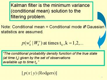
Kalman filter is the minimum variance
(conditional mean) solution to the filtering
problem.
Note Conditional mean Conditional mode if
Gaussian statistics are assumed.
The conditional probability density function of
the true state (at time tk) given by the set of
observations available up to time tk.
2
Lets assume we already understand the
stochastic dynamic and stochastic observation
models and begin from there.
Equations 2.9 and 2.13 (Cohn) or 7.3 and 7.4
(Rodgers).
Warning Cohn uses a subscript k to refer to
time index and a superscript t to refer to
truth. Rodgers uses a subscript t to refer
to the time index. As we go along I will
attempt to clarify both notations. Cohn (section
2) does a good job deriving these equations.
3
Discrete Stochastic Dynamic Model
Discrete true state
Discrete propagator (evolves state from previous
time)
Model error (generally continuum
state-dependent) We will assume a mean and
covariance to represent this term.
4
Discrete Stochastic Observation Model
Observation of continuum state at times tk,
k1,2,
Discrete forward observation operator
Total observation error includes both
measurement error and error of representativeness
(i.e. error d/t acting upon discrete state
instead of a continuous one.)
5
Probabilistic Assumptions of Discrete Kalman
Filter
Propagator (fk) and observation operator (hk) are
linear. (Denoted now as Fk and Hk)
6
Multivariate Gaussian Distribution
N Normal Distribution (Gaussian)
Mean alpha
Covariance Qk
White (random signal -gt equal power at any band)
7
Take a closer look at the dynamic model.
1. Do we know the discrete true state?
No! We must make a prediction of it. This is
done during the forecast step of the Kalman
filter.
2. The Kalman filter is recursive. Knowledge of
a prior estimate of the state mean and error
covariance is required.
8
Forecast Step
We need to predict an expected value of the true
state given all previous observations (as well
as a forecast error covariance matrix).
(Eq) 4.5
Substitute in for the stochastic dynamic model
and solve.
0 Why?
Why are F and G outside expectation operator?
9
Forecast Step (2)
(Eq) 4.6
Substitute in for the stochastic dynamic model
and expected forecast state and solve.
Like previous slide, cross terms vanish due to
Probabilistic Assumptions. (Stochastic state
and observation error is Gaussian (with mean0)
and white.
10
Sowhat just happened?
We just calculated our prior. The
probability of the current true (discrete) state
given all previous observations.
11
Each updated state estimate and error covariance
becomes the prior knowledge at the following
time step (green arrows).
Note Equation numbers do not refer to Cohn paper
or Rodgers book on this slide.
12
Getting from A to B
Prior
Solution to Filtering Problem
Use definition of conditional probability
densities. (See Cohn Appendix A or any
probability theory text)
13
Bayes Theorem
Prior
(Eq) 4.13
Something
We still need to calculate 2 probability
densities on RHS (by using the (discrete)
stochastic observation model).
(Eq) 2.19 Rodgers
14
Just like we did for the prior, define a
expected value and error covariance matrix and
substitute in for observation model.
0 Observation error NOT state dependent and mean
error 0 (by probabilistic assumptions).
Mean
(Eq) 4.14
(Eq) 4.15
Error Covariance
Create Gaussian distribution using this mean and
covariance. Compare to Rodgers (Eq) 2.21
Must be Gaussian because observation error
assumed to be Gaussian!!
15
Define an expected value and error covariance
matrix and substitute in for observation model.
0 (Observation error is white).
Mean
(Eq) 4.16
Error Covariance
Cross terms vanish due to probabilistic
assumptions. Note (AB)TBTAT
(Eq) 4.18
Must also be Gaussian because observation error
assumed to be Gaussian!!
16
1. We now have all information needed to
calculate the solution to our filtering problem.
2. Using mean and covariance for each term on
RHS, create a Gaussian distribution equation
(refer to earlier slide for the multivariate
Gaussian equation and equations 4.20-4.22 of
Cohn).
For example, Something can be written as
17
3. Manipulate terms to the following form. In
order to maximize the probability of the state
given all observations available up to the
current time, you must minimize J.
(Eq) 4.25
(Eq) 4.24
4. Our final goal is to derive a mean and
covariance matrix for the final probability
density. This requires matrix manipulations,
substitutions, etc involving J.
Refer back to slide 8 and analysis mean and
covariance equations.
18
Analysis Update Equations
(Note Equations 4.26-4.42 rigorously derive
these equations.)
(Eq) 4.43-4.45
Kalman Gain matrix
The Kalman Gain matrix distributes the difference
between the current observation and the a priori
estimate of the field amongst the state variables.
19
Lets look at a couple of limits on the Kalman
gain matrix
1. Large measurement noise (large Rk) -gt small Kk
and measurement is weighted only slightly. In
limit of infinitely noisy measurements, new
measurement info is totally ignored and the new
estimate for the state equals the apriori
information.
2. Large uncertainty in dynamic model (large Pf)
-gt large Kk and new measurement is weighted
heavily.
20
Lets look closer at the analysis update error
covariance
(Eq) 4.26
Take inverse
GOOD NEWS!! Note that the analysis error
covariance is smaller than both the forecasted
error covariance and the observation
error covariance!!
21
Kalman Filter Equations
Forecast Equations
Analysis Update Equations
Equations 7.5-7.9 represent Rodgers form.
Reference slide also available at end of
presentation.
22
Green arrows path of forecast equations
Discrete Propagator
Analysis Update Equations
Discrete Forward Observation Operator
Note Equation numbers do not refer to Cohn paper
or Rodgers book on this slide.
23
Truth random walk with variance1 Measurement
Variance is Gaussian with mean0, and
std.dev2. M 1 (persistence) (i.e. forecast) K
1 (direct observations) (forward observation
operator)
Simple Example (Rodgers terminology)
24
Example 2 A Study of Kalman Filtering Using
Hypothetical HIRDLS Data (again using Rodgers
notation).
1. Temperature data was represented as a Fourier
series (discrete forward observation operator)
2. Fourier series is a linear combination of
standing waves.
Temp.
Wavenumber index
Longitude location
Coefficients of zonal Fourier Expansion (i.e.
state vector)
Mean temp. of latitude band
25
3. Goal was to determine the increase in accuracy
(of temperature amplitudes and phases) that
could be achieved when using Kalman filter
equations on high density HIRLDS data
(hypothetical) compared to lower density data.
(LRIR study in 1981 illustrated Kalman
filter Equations could accurately retrieve
Fourier coefficient Representation of
temperature up through wavenumber6.)
The discrete operator used was persistence.
26
(No Transcript)
27
(No Transcript)
28
(No Transcript)
29
Comparison 133hPa, 60N
Amplitude (K)
30
Amp. Diff. Plots 133hPa, 60N
(a)
Amplitude (K)
(d)
31
Phase Diff. Plots 133hPa,60N
(a)
(b)
32
Error Covariance Matrix-6swath
14
0
2
Wavenumber
.0
14
33
Kalman Filter Equations(Rodgers format)
Bold face indicates a matrix.
34

• References
• Cohn, S.E., 1997 An Introduction to Estimation
  Theory. J Met. Soc. Japan, 75, 257-288.
• Rodgers, C., D., 2000 Inverse methods for
  atmospheric sounding theory and practice. World
  Scientific Computing.