The Breeding Method

1
Ocean Instabilities Captured By Breeding On A
Global Ocean ReanalysisOS11B-1482
For more information, contact Matthew
Hoffman, Mathematics Building University of
Maryland College Park, MD 20742 Tel.
301-405-8735 E-mail mhoffman_at_math.umd.edu
Matthew J. Hoffman1, James Carton2, Eugenia
Kalnay2, and Shu-Chih Yang2 1Department of
Applied Mathematics, University of Maryland,
College Park, Maryland 2Department of Atmospheric
and Oceanic Sciences, University of Maryland,
College Park, Maryland
Abstract The breeding method, which has
previously been applied to atmospheric and even
coupled models, is implemented on a global ocean
reanalysis for the purpose of isolating
instabilities of the system. We performed
breeding experiments with the GFDL Modular Ocean
Model (MOM) and have obtained bred vectors
related to both tropical instability waves and
ENSO, among other processes. By varying the
length of the time between rescaling and the
scale factor used, different instabilities can be
made dominant in the bred vector. These bred
vectors have potential applications in oceanic
data assimilation and ensemble forecasting
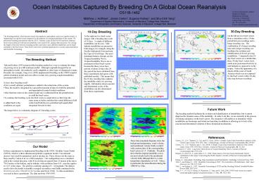
30-Day Breeding On the left are two bred vectors
from a simulation with a 30-day period between
rescalings and a larger rescaling size. The
combination of a longer rescaling time and a
larger rescaling size facilitates the isolation
and identification of slower growing
instabilities. Compared to the 10-day bred
vectors on a similar date, these 30-day bred
vectors show much more pronounced activity in
mid-latitudes as opposed to in the tropics.
Notice the appearance of a dipole off the coast
of South America which was not captured by the
bred vectors with a 10-day time step between
rescalings.
10-Day Breeding To the right are two bred vector
images with a breeding time scale of 10 days. A
couple of different instabilities can be seen.
Mid-latitude instabilities are present in both
images, for example, along the Pacific
Subtropical Front and near the Cape of Good Hope.
The most dominant features, though, are the
Tropical Instability Waves. Tropical Instability
Waves are so prominent in these bred vectors
because the these waves have periods of about 20
days (the 20 day period has been calculated from
these experiments and agrees with published
results). This means that the 10 day rescaling
time captures the instability while it is growing
rapidly. Information about seasonal and
interannual cycles of the instabilities can also
determined from these experiments.

• The Breeding Method
• Toth and Kalnay (1993) proposed the breeding
  method as a way to estimate the shape of growing
  errors in a full nonlinear model. Although
  originally designed for an atmospheric model,
  the method is easily adaptable to other types of
  dynamical systems. Recently, for example, Yang et
  al. (2006) implemented breeding on the NSIPP
  coupled global circulation model and were able to
  isolate slow growing coupled instabilities
  associated with ENSO.
• So how does breeding work?
• First, a small, arbitrary perturbation is added
  to the initial state of the system.
• Then, the model is integrated for a prescribed
  amount of time for both the perturbed and
  unperturbed (control) initial conditions.
• After that time interval, the control model run
  is subtracted from the perturbed run to yield
  the bred vector.
• To continue the breeding cycle, the bred vector
  is scaled down so that it has the same norm as
  before and then this scaled difference field is
  added back to the control and both the new
  perturbed and unperturbed conditions are again
  integrated forward in time.
• The image below is a schematic diagram of 5
  breeding cycles.

Future Work The breeding method facilitates the
isolation and identification of instabilities,
but it cannot diagnose the dynamic cause of the
instability. In order to do this, we are
currently in the process of running energetics on
the bred vectors. The energetics will enable us
to determine which instabilities are barotropic
and which are baroclinic in addition to allowing
us to look at the seasonal and interannual
variation of these dynamical mechanisms.
References Carton, J.A., G.A. Chepurin, X. Cao,
and B.S. Giese, 2000a A Simple Ocean Data
Assimilation Analysis of the
Global Upper Ocean 1950-1995, Part 1
Methodology. Journal of Physical Oceanography,
30, 294-309. Carton, J.A., G.A. Chepurin, and X.
Cao, 2000b A Simple Ocean Data Assimilation
Analysis of the Global Upper Ocean
1950-1995 Part 2 Results. Journal of Physical
Oceanography, 30, 311-326. Contreras, R. F. 2002
Long Term Observations of Tropical Instability
Waves. Journal of Physical
Oceanography, 32, 2715-2722. Halpern, D., Knox,
R. A., and Luther, D. S., 1988 Observations of
20-Day Period Meridional Current
Oscillations in the Upper Ocean along the Pacific
Equator. Journal of Physical Oceanography, 18,
1514-1534. Kalnay, E. Atmospheric
Modelling, Data Assimilation and Predictability,
Cambridge University Press, 2003. Toth, Z., and
Kalnay, E., 1993 Ensemble Forecasting at NMC
The Generation of Perturbations. Bull. Amer.
Meteorol. Soc, 74, 2317-2330. Toth, Z.,
and Kalnay, E., 1997 Ensemble Forecasting at
NCEP and the Breeding Method. Monthly Weather
Review, 125, 3297-3319. Yang, S.-C., M.
Cai, E. Kalnay, M. Rienecker, G. Yuan, and Z.
Toth, 2006 ENSO bred vectors in coupled
ocean-atmosphere general circulation models. J.
Clim., 19, 1422-1436
Courtesy of Shu-Chi Yang
These time-longitude diagrams show the background
temperature, zonal velocity, and meridional
velocity fields overlaid with contour plots of
the corresponding bred vectors at 3.5N latitude.
The plots show that the tropical instability
waves are most closely tied to the meridional
velocity field, although there is a clear
temperature dependence as well. Notice, in
particular, the intensification during the
1988-89 La Niña.
Our Model In these experiments we implemented
breeding on the GFDL Modular Ocean Model (MOM),
which is a three-dimensional primitive equations
model. Conventional choices were used for
parameters such as mixing, etc. These choices are
the same as those used by Carton et al. in a 2000
reanalysis. Our configuration uses a stretched
grid in the vertical direction, with 20 levels
that are spaced from 15 meters at the top to
736.9 meters at the bottom, and in latitude, with
resolution from 0.43 near the equator to 1.02
at the edges. The grid has a uniform spacing of
1 in longitude. The dataset used to drive the
model is monthly averaged sea-surface wind fields
contained in the World Ocean Atlas 1994 (WOA-94
Levitus and Boyer 1994). No data assimilation
was used in these experiments. The data ran from
1950-1995.