Flare Rate Analysis of M Dwarf Light Curves

1
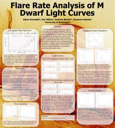
Flare Rate Analysis of M Dwarf Light Curves
Adam Kowalski1, Eric Hilton1, Andrew Becker1,
Suzanne Hawley1
1University of Washington
Abstract M Dwarfs produce intense flares from
a magnetic dynamo that is not completely
understood. Since M Dwarfs dominate the
celestial census, M Dwarf flares must be
distinguished from variable objects of interest
to next generation time domain surveys, such as
LSST. We present a representative sample of
flaring candidates from 7,621 M Dwarf photometric
light curves extracted from the Sloan Digital Sky
Surveys Equatorial Stripe. We estimate a
variability index for discriminating flaring
epochs from non-flaring epochs. We also present
preliminary trends of flaring rates as a function
of spectral type and magnetic activity.
Example Flare Spectrum
Equatorial Stripe Population
Figure 1 Example of an M star in both flaring
(red) and quiescent (black) states normalized at
8000 Å. The Sloan Filter central wavelengths are
indicated. Notice that in the flaring state, the
hydrogen lines are strongly in emission and that
the blue continuum flux increases. Although the
u-filter is only partially shown, it is obvious
that the ratio of flare-to-quiescient flux is
greater in the u-filter than the g-filter.
Light Curves Light curves with high variability
index (gt400)
Figure 4 Top center - Number of M stars per
spectral class for different magnetic activity
levels Active (red), Non-Active (black), and
Weakly Active (dashed line). Active stars are
typically later spectral type. Bottom - Number
of M stars that flare per spectral class for
different magnetic activity levels Active
Weakly Active (red) and Non-Active (black).
Bottom left plots the number of flares as defined
by I gt 400 and .
Bottom right plots the number of flares as
defined by Igt200 and .
Active star flares occur at a later spectral
type than non-active star flares. Since our
sample contains many more non-active early type
stars (top center), we expect to see a higher
number of non-active early type star flares.
Technique Sample Our sample consists of 7,621 M
Dwarf objects (subclassed by magnetic activity
and spectral type) with an average of 20
epochs/object. Each object has photometric data
in 5 filters u, g, r, i, z. Photometric Tests
We test all of the epochs for good and bad
photometry in the u- and g-filters. Variability
Tests For the epochs in which the u- and
g-filters have good photometry, we calculate a
Variability Index to determine whether the
epochs flux in both the u- and g-filters
increases significantly enough to be considered a
flare. We use a modified version of the Welch
Stetson (1993) variability index
Light curves with intermediate variability index
(200 to 400)
We use two thresholds to define a high
variability and intermediate variability
Flaring Fraction

• High Variability Index I gt 400
• Intermediate Variability Index I gt200

Flux Ratio Test From Figure 1, we expect flares
to increase the flux in the u-filter the most.
Therefore, a flare must also satisfy
Figure 3 The flux ratio (
) vs. epoch number for the u-filter (blue) and
g-filter (red) for a representative sample of
flare candidate light curves. The light curves
are labeled with spectral type and magnetic
activity. We selected these light curves as
flaring candidates because one or more epochs
have a high (top) or an intermediate (bottom)
variability index and
because we expect that flares produce the
largest increase in the u-filter flux (see Figure
1). Note that the continuous trends are meant
to guide the eye and that the upward spikes are
defined by a single data point.
Time Sampling
Figure 5 Since our sample contains more early
type stars, we calculated the flaring fraction
per spectral type for active stars (red) and
non-active stars (black). The flaring fraction is
flaring epochs / total epochs. We define
flares the same way as above with the high
variability index shown on the left and the
intermediate variability index shown on the
right. Figure 4 shows that the number of flaring
stars (active non-active) is greatest at early
types however, Figure 5 shows that the flaring
fraction increases at later spectral type.
References

• Welch, D. L. Stetson, P. B. Astr. J. 105, 1813
  (1993)

Figure 2 The times at which photometry was
taken relative to the time of the first
observation. Every 100th object in our sample is
plotted along the y-axis. There are clusters of
observations separated widely in time over 6
years.