
Physical Climate Models - PowerPoint PPT Presentation
Title:
Physical Climate Models
Description:
Models may handle radiative transfers in detail but neglect or parameterize ... Models may provide 3-D representation but contain much less detailed radiative ... – PowerPoint PPT presentation
Number of Views:217
Avg rating:3.0/5.0
Title: Physical Climate Models
1
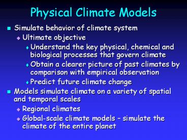
Physical Climate Models
- Simulate behavior of climate system
- Ultimate objective
- Understand the key physical, chemical and
biological processes that govern climate - Obtain a clearer picture of past climates by
comparison with empirical observation - Predict future climate change
- Models simulate climate on a variety of spatial
and temporal scales - Regional climates
- Global-scale climate models simulate the
climate of the entire planet
2
Climate Processes
- Three processes that must be considered when
constructing a climate model - 1) radiative - the transfer of radiation through
the climate system (e.g. absorption, reflection) - 2) dynamic - the horizontal and vertical transfer
of energy (e.g. advection, convection,
diffusion) - 3) surface process - inclusion of processes
involving land/ocean/ice, and the effects of
albedo, emissivity and surface-atmosphere energy
exchanges
3
Constructing Climate Models
- Basic laws and relationships necessary to model
the climate system are expressed as a series of
equations - Equations may be
- Empirical derivations based on relationships
observed in the real world - Primitive equations that represent theoretical
relationships between variables - Combination of the two
- Equations solved by finite difference methods
- Must consider the model resolution in time and
space i.e. the time step of the model and the
horizontal/vertical scales
4
Simplifying the Climate System
- All models must simplify complex climate system
- Limited understanding of the climate system
- Computational restraints
- Simplification may be achieved by limiting
- Space and time resolution
- Parameterization of the processes that are
simulated
5
Model Simplification
- Simplest models are zero order in spatial
dimension - The state of the climate system is defined by a
single global average - Other models include an ever-increasing
dimensional complexity - 1-D, 2-D and finally to 3-D models
- Whatever the spatial dimension, further
simplification requires limiting spatial
resolution - Limited number of latitude bands in a 1-D model
- Limited number of grid points in a 2-D model
- Time resolution of climate models varies
substantially, from minutes to years depending on
the models and the problem under investigation - To preserve computational stability, spatial and
temporal resolution must be linked - Can pose problems when systems with different
equilibrium time scales have to interact as a
very different resolution in space and time may
be needed
6
Parameterization
- Involves inclusion of a process as a simplified
function rather than an explicit calculation from
first principles - Sub-grid scale phenomena, like thunderstorms,
must be parameterized - Not possible to deal with these explicitly
- Other processes are parameterized to reduce
computation required - Certain processes omitted from model if their
contribution negligible on time scale of interest - Role of deep ocean circulation while modeling
changes over time scales of years to decades - Models may handle radiative transfers in detail
but neglect or parameterize horizontal energy
transport - Models may provide 3-D representation but contain
much less detailed radiative transfer information
7
Modeling Climate Response
- Ultimate purpose of a model
- Identify response of the climate system
- Change in the parameters and processes that
control the state of the system - Climate response occurs to restore equilibrium
within the climate system - If radiative forcing associated with an increase
in atmospheric CO2 perturbs the climate system - Model will assess how the climate system responds
to this perturbation to restore equilibrium
8
Model Equilibrium
- Model may require many years of simulated change
to reach equilibrium - Final years of simulation averaged
9
Nature of the Model
- One of two modes
- Equilibrium mode
- No account taken of energy storage processes that
control evolution of climate response with time - Assume climate responds instantaneously following
system perturbation - Transient mode
- Inclusion of energy storage processes
- Simulate development of a climate response with
time - Models typically run twice
- In a control run with no forcing
- In a test run including forcing and perturbation
of the climate system
10
Climate Sensitivity
- Critical parameters
- In the most complex models
- Climate sensitivity calculated explicitly through
simulations of processes involved - In simpler models
- Climate sensitivity is parameterized by reference
to the range of values suggested by the more
complex models - This approach, where more sophisticated models
are nested in less complex models, is common in
the field of climate modeling
11
Data-Model Comparisons
- Models constructed to simulate Modern circulation
- Changes based on Earth History inserted in model
- Climate output compared with observations
12
One-Dimensional Models
- Simplified representation of of entire planet
- Model driven by global mean incoming solar
radiation and albedo - Single vertical column of air divided into layers
- Each layer contains important constituents (dust,
greenhouse gases, etc) - Layers exchange only vertically
13
Types of Models
- Energy balance models (EBMs)
- Simulate two fundamental climate processes
- Global radiation balance
- Latitudinal (equator-to-pole) energy transfer
- Radiative-convective models (RCMs)
- Simulate detailed energy transfer through the
depth of the atmosphere - Radiative transformations that occur as energy is
absorbed, emitted and scattered - Role of convection
14
EBMs
- 0-D EBMs
- Earth is a single point in space
- Global radiation balance modeled
- In 1-D models latitude is included
- Temperature for each latitude band is calculated
- Using latitudinal value for albedo, energy flux,
etc. - Latitudinal energy transfer estimated from linear
empirical relationships - Difference between latitudinal temperature and
global average temperature
15
RBMs
- Surface albedo, cloud amount and atmospheric
turbidity - Used to determine heating rates atmospheric
layers - Imbalance between net radiation at top and bottom
of each layer determined - If calculated vertical temperature profile (lapse
rate) exceeds some stability criterion (critical
lapse rate) - Convection is assumed to take place (i.e. the
vertical mixing of air) until the stability
criterion is no longer breached
16
Two-Dimensional Models
- Multi-layered atmosphere coupled with Earths
physical properties averaged by latitude - Allows simulations of climatic processes that
vary with latitude - Angle of incoming solar radiation
- Albedo of Earths surface
- Heat capacity changes
17
Statistical-Dynamical Models
- Combine horizontal energy transfer modeled by
EBMs with the radiative-convective approach of
RCMs - Equator-to-pole energy transfer is more
sophisticated - Parameters like wind speed and wind direction
modeled by statistical relations - Laws of motion are used to obtain a measure of
energy diffusion - Particular useful to investigate role of
horizontal energy transfer and processes that
directly disturb that transfer
18
2-D Models
- Advantage
- Simulate long intervals of time quickly and
inexpensively - Disadvantage
- Not sensitive to climate processes that depend on
geographic position of continents and oceans
19
Three-Dimensional Models - GCM
- 3-D representation of Earths surface and
atmosphere - Most sophisticated attempt to simulate the
climate system - 3-D model based on fundamental laws of physics
- Conservation of energy
- Conservation of momentum
- Conservation of mass
- Ideal Gas Law
20
GCMs
- Represent key features affecting climate
- Spatial distribution of land, water, ice
- Regional variation in heat capacity and albedo of
surface - Elevation of mountains and glaciers
- Concentrations of greenhouse gases
- Seasonal variations in solar radiation
- Calculations at interactions of grid boxes
21
GCMs
- Atmospheric variables at each grid point requires
the storage, retrieval, recalculation and
re-storage of 105 figures at every time-step - Models contain thousands of grid points
- GCMs are computationally expensive
- Can provide accurate representations of planetary
climate - Simulate global and continental scale processes
in detail - GCMs cannot simulate synoptic regional
meteorological phenomena (e.g.,tropical storms) - Play an important part in the latitudinal
transfer of energy and momentum - Spatial resolution of GCMs limited in vertical
dimension - Many boundary layer processes must be
parameterized
22
Sensitivity Test
- Control case established
- Modern climate simulated
- One boundary condition altered at a time
- Model output compared with present day climate
simulation - Information reveals impact of that boundary
condition - Boundary condition examples
- Continental configuration
- Ice sheet expansion
- Solar radiation influx
- Greenhouse gas concentrations
23
Model Resolution
- Can it image New Zealand? this is probably now
out of date! (2 lat x 3 long)
24
Atmospheric and Ocean GCMs
- Atmospheric GCM more sophisticated
- Much detail known about atmospheric circulation,
elevations, landmasses, etc. - Ocean GCM primitive
- Rudimentary knowledge of oceanic circulation
- Deep water formation
- Difficult to model important small features
- Fast-moving narrow currents
25
Oceanic GCMs
- Similar in construction to atmospheric GCM
- Lower boundary seafloor
- Water column divided grid boxes
- Low resolution, fewer layers/boxes, biology
- Output temperature, salinity, sea ice, gases
26
Atmospheric and Ocean GCMs
- Oceanic GCMs simulates circulation over several
years to decades - Atmospheric GCMs simulates circulation over
several hours to weeks - Basic incompatibility between models
- A-GCMs may be used to drive O-GCMs
- Asynchronous coupling
- Atmospheric conditions drive ocean
- Oceanic conditions drive atmosphere
- Alternation keeps systems from getting wacky
27
Geochemical Models
- Mass balance models
- Follow movement of Earth materials from one
reservoir to another - Physical or chemical form
- Models focus on sources, rates of transfer and
depositional fate of materials - Commonly trace fate of materials using a
geochemical tracer - Example 18O content of seawater
28
One-way Mass Transfer Models
- Movement from source to sink
- Movement from one reservoir to another
- If materials transferred has unique chemical or
physical signature - Flux rate (mass transfer time-1) can be
determined - Example calving of icebergs
- Influx of ice-rafted debris
- Determined by physical sedimentology
- Quantified by point-counts
29
Mass Balance Equations
- Simple mass balance
- Ftotal F1 F2 F3
- Tracer mass balance
- TR (F1T1 F2T2 F3T3)/(F1 F2 F3)
- TR is the mean value of tagged inputs
- Mass balance of two components in system
- Tracer entering tracer leaving
- TR ƒinTin (1 ƒout)Tout
30
Tracer Mass Balance Example
- Global carbon redox balance
- Average d13C of carbon on Earth -4.6
- CO2 in hydrothermal vents
- Average d13C of carbonates 0.6
- Average d13C of organic carbon -25.4
- Know
- 13C entering 13C leaving
- dR ƒodo (1 ƒo)dcarb
- 4.6 ƒo(-25.4) (1 ƒo)0.6
- 20 of carbon buried in marine sediments is
organic carbon
31
Chemical Reservoirs
- Earth reservoirs
- Atmosphere, ocean, ice, vegetation and sediments
- Ocean most important reservoir
- Interacts with other reservoirs
- Receives weathering products
- New minerals deposited in sediments
- Tracer is carried to ocean, mixed and trapped in
sedimentary mineral archive
32
Steady State Tub
- If flux of tracer into and out of reservoir are
equal, the system is at steady state
33
Residence Time
- Time it takes for tracer to pass through tub
- Residence time reservoir size/flux
- Residence time of tracer typically gt mixing time
of the ocean (1500 y) - Tracer distribution homogenous
- Tracer concentration or isotopic composition is
everywhere equal - Records whole-ocean chemistry during deposition
34
Reservoir Exchange Models
- Models can be designed to track reversible
exchange between different sized reservoirs
35
Reservoir Exchange
- Monitor cycling of tracers between reservoirs
through time - Tracer with distinctive value moves freely
between reservoirs - Typically between small and large reservoirs
- Ocean and atmosphere, vegetation, land
- Monitors change in size of smaller reservoir
- Tracer exchange detected in sedimentary minerals
- Exchange produces change in volume and tracer
value in ocean
36
Reservoir Exchange Example
- Change in the d18O of seawater
- d18O of glacial ice and seawater different
- Change in glacial ice volume
- Produces small changes in the oxygen isotopic
composition of seawater - Change in seawater d18O recorded
- Calcareous shells or sediment porewater
- Glacial ice small reservoir and ocean large
reservoir
37
Time-Dependent Models
- Most geochemical models assume steady-state
conditions - Time-dependent models assume steady-state only
during equilibrium conditions - Steady-state conditions imply no change in
reservoir size - Time-dependent models allow changes in reservoir
size - From one equilibrium state to another
- Under equilibrium
- Steady-state conditions prevail
38
CO2 and Long-Term Climate
- What has moderated Earth surface temperature over
the last 4.55 by so that - All surface vegetation did not spontaneously
catch on fire and all lakes and oceans vaporize? - All lakes and ocean did not freeze solid?
39
Greenhouse Worlds
- Why is Venus so much hotter than Earth?
- Although solar radiation 2x Earth, most is
reflected but 96 of back radiation absorbed
40
What originally controlled C?
- In solar nebula most carbon was CH4
- Lost from Earth and Venus
- Earth captured 1 in 3000 carbon atoms
- Tiny carbon fraction in the atmosphere as CO2
- 60 out of every million C atoms
- Bulk of carbon in sediments on Earth
- CaCO3 (limestone and dolostone) and organic
residues (kerogen) - Venus probably had similar early planetary
history - Most carbon is in atmosphere as CO2
- Venus has conditions that would prevail on Earth
- All CO2 locked up in sediments were released to
the atmosphere
41
Earth and Venus
- Water balance different on Earth and Venus
- If Venus and Earth started with same components
- Venus should have either
- Sizable oceans
- Atmosphere dominated by steam
- H present initially as H2O escaped to space
- H2O transported "top" of the Venusian atmosphere
- Disassociated forming H and O atoms
- H escaped the atmosphere
- Oxygen stirred back to surface
- Reacted with iron forming iron oxide
42
Planetary Evolution Similar
- Although Earth and Venus started with same
components - Earth evolved such that carbon safely buried in
early sediments - Avoiding runaway greenhouse effect
- Venus built up CO2 in the atmosphere
- Build-up led to high temperature
- High enough to kill all life
- If life ever did get a foothold
- Once hot, could not cool
43
Why Runaway Greenhouse?
- Don't know why Venus climate went haywire
- Extra sunlight Venus receives?
- Life perhaps never got started?
- No sink for carbon in organic matter
- Was the initial component of water smaller than
that on Earth? - Did God make Venus as a warning sign?
44
Early Earth Faint Young Sun
- Solar Luminosity 4.55 bya 25 lower than today
- Faint young Sun paradox
- If early Earth had no atmosphere or todays
atmosphere - Radiant energy at surface well below 0C for
first 3 billion years of Earth history - No evidence in scant Archean rock record that
planet was frozen
45
Early Earth A Greenhouse World
- Earth was more Venus-like during Archean
- Models indicate that greenhouse required
- Several greenhouse gases
- H2O, CO2, CH4, NH3, N2O
- H2O and CO2 most likely
- 102-103 x PAL CO2
46
Archean Atmosphere
- Faint young Sun paradox presents dilemma
- 1) What is the source for high levels of
greenhouse gases in Earths earliest atmosphere? - 2) How were those gases removed with time?
- Models indicate Suns strength increased slowly
with time - Geologic record strongly suggests Earth
maintained a moderate climate throughout Earth
history (i.e., no runaway greenhouse like on
Venus)
47
Source of Greenhouse Gases
- Input of CO2 and other greenhouse gases from
volcanic emissions - Most likely cause of high levels in Archean