Atmospheric Chemistry Measurement and Modeling Capabilities are Advancing on Many Fronts

1
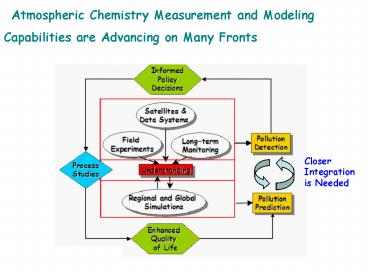
Atmospheric Chemistry Measurement and Modeling
Capabilities are Advancing on Many Fronts
Closer Integration is Needed

2
Predictability as Measured by Correlation
Coefficient Met Parameters are Best
lt 1km
O3 predicted better than CO
Performance decreases with altitude
Carmichael et al., JGR, 2003
3
Model vs. Observations

• Cost functional measures the model-observation
  gap.
• Goal produce an optimal state of the atmosphere
  using
• Model information consistent with
  physics/chemistry
• Measurement information consistent with reality
• All with errors

Modeled O3 vs. Measured O3
4
Challenges in chemical data assimilation

• A large amount of variables (100 concentrations
  of various species at each grid points)
• Memory shortage (check-pointing required)
• Various chemical reactions (gt200) coupled
  together (lifetimes of different species vary
  from seconds to months)
• Stiff differential equations
• Chemical observations are very limited, compared
  to meteorological data
• Information should be maximally used, with least
  approximation
• Highly uncertain emission inventories
• Inventories often out-dated, and uncertainty not
  well-quantified

5
Data assimilation methods

• Simple data assimilation methods
• Nudging
• Optimal Interpolation (OI)
• 3-Dimensional Variational data assimilation
  (3D-Var)
• Ensembles
• Advanced data assimilation methods
• 4-Dimensional Variational data assimilation
  (4D-Var)
• Fisher and Lary (1995), AutoChem model
• CTMs with 4D-Var applications STEM, EURAD,
  CHIMERE
• Kalman Filter (KF)
• Many variations, e.g. Ensemble Kalman Filter
  (EnFK)
• CTMs with KF applications EUROS, LOTOS, MOZART,
  EURAD

6
Extensive Real-Time Evaluation of Regional
Forecasts Stu McKeen
http//www.etl.noaa.gov/programs/2004/neaqs/verifi
cation/
7
Forecast Skill (Persistence vs Model)
STEM-2K3
Persistence
8
Forecast Skill (One Model vs Ensemble)
Ensemble (8 models)
One CTM model
9
Ensemble Techniques Help
10
4D-Var data assimilation
dx
(new)
(initial condition for NWP)
(old forecast)
11
4D-Var application with CTMs
12
Variational Data Assimilation Using Adjoints
(4dVar)
e.g., emissions
13
Our Analysis Framework
Influence Functions Emission Biases/ Inversion
Mesoscale Meteorological Model (RAMS or MM5)
MOZART Global Chemical Transport Model
Anthropogenic biomass burning Emissions
Meteorological Dependent Emissions (biogenic,
dust, sea salt)
TOMS O3
STEM Prediction Model with on-line TUV SCAPE
STEM Tracer Model (classified tracers for
regional and emission types)
STEM Data- Assimilation Model
Chemistry Transport Analysis
Airmasses and their age intensity Analysis
Observations
14
Assimilation of AIRNOW O3 surface observations
for July 20, 2004 adjusts predictions considerably
Observations circles, color coded by O3 mixing
ratio
Surface O3 (forecast)
Surface O3 (analysis)
15
Assimilation of elevated observations for July
20, 2004
Ozonesonde observations (Rhode Island)
NOAA P3 flight observations
16
Getting the Vertical Distributions Right is
Critical
Current models have a difficult timeso data
assimilation is important
IONS O3 data Anne Thompson John Merrill
17
Change of Initial O3 after Assimilation

• Date
• July 20, 2004
• Observations
• AirNow, P3-O3, Ozonesonde
• Isosurfaces of relative changes
• -20 (blue), 20 (yellow), 100 (red)

18
Effect of Assimilation on Forecast
19
Courtesy John Reilly, MIT
20
A Key Issue Is Which Data To Assimilate --
Example Impact of Assimilating NOy
Leads to improved prediction of NO, NO2, PAN, and
HNO3
21
Simultaneous Assimilation of Multiple Species
22
CO assimilation with CO as control (left) and
with various VOCs as added controls (right)
23
We Plan to Include LIDAR and MOZAIC Data
Difference
24
Modeling the Background Error Term

• AR Models
• Improved 4D-Var Results

25
4d-Var data assimilation results are visibly
improved when using the new AR background
covariance
Observation error 8 I.C. error 10ppbv Initial
ozone is control
Tacoma, DC
McMillian Reservoir, DC
26
Station 3
12 EDT July 21 w/o (top) and w (bottom)
assimilation
12 EDT July 20 (w/o (top) and w (bottom)
assimilation)
27
Ensemble-based Chemical Data Assimilation

• Formulation and Challenges
• Examples

28
Experimental setting of the ensemble-based data
assimilation system

• 50 members, perturbed I.C., B.C., and emissions
• 30 initial std, AR correlations TESV
  perturbations
• O3 and NO2 observations at 24 ground locations in
  3 countries, and in one vertical column.
  Perturbation 0.1 std, uncorrelated
• Quality of analysis in a sub-domain including
  observation sites

29
Ensemble data assimilation is effective when the
initial ensemble is based on TESV perturbations
50 members (TESVbckg), 24 hrs., 30 initial std,
24 ground, 1 column O3NO2 obs. sites, 0.1 obs.
std.
O3
NO2
30
Effect of Dry Deposition on Ozone Forecast
31
Where do we go from here?Example of Use of 3-D
CFORS modeling system at TRACE-P Information Day
in Hong Kong
We need better decoder glasses
32
Effects of Physical Removal Processes which are
significant sources of uncertainty
High Dry Dep Case Change in surface ozone (ppb)
With/W-o wet dep Change in column BC
33
Improving Emissions is a Top Priority Models,
Emissions, and Observations are not Perfect
Inverse Modeling
34
4dVar can be used to recover emissions
k
Forward
Inverse
35
Chemical Data Assimilation The Future?

• Feasible necessary.
• Just the beginning more ??s than answers but
  we have test beds!
• Important implications for measurement systems
  and models.
• Need to grow the community.

36
Air Quality Analysis A Challenge of Scales and
Integration
Requires Close Integration of Observations and
Models
Pierce NASA/Langley
37
(No Transcript)
38
(No Transcript)
39
(No Transcript)
40
(No Transcript)
41
Atmospheric chemical data assimilation
Meteo model
Optimal analysis state
Chemical model
CTM
Observations
Data Assimilation
Forecast
Aerosol model
Emissions
Targeted observ.
42
Dynamic data driven simulations of atmospheric
chemistry, particles, and transport are
challenging
43
Assimilated chemical observations

• Field campaign measurements
• TRACE-P, ACE-ASIA, ICARTT, GOME, and HALOE
  (aircraft, ship, and surface station measurements
  of various species)
• Surface monitoring net-work
• CMDL (CO), AIRNOW(O3), AIRPARIF (O3)
• Satellite data
• UARS (Ozone, NO2), MOPITT (CO)
• Other data
• MOZAIC (Measurements of OZone and water vApor by
  airbus In-service airCraft)

44
4D-Var Data Assimilation Results

• Parallel Adjoint STEM
• ICARTT Results

45
ICARTT field campaign in Eastern U.S., July 2004
46
Ensemble-based chemical data assimilation
techniques can complement the variational tools

• Motivation
• Ensemble-based d.a. generate a statistical sample
  of analyses
• Explicitly propagate (approximations of) the
  error statistics
• Can deal effectively with nonlinear dynamics
• Complement variational techniques
• Issues
• Initialization of the ensemble
• Rank-deficient covariance matrix
• Contributions
• Models of background error covariance
• Calculation of TESVs for reactive flows
• Targeted observations using TESVs
• Ensemble-based assimilation results

47
Ensemble data assimilation improves the
prediction of species which are not directly
observed
50 members (TESVbckg), 24 hrs., 30 initial std,
24 ground, 1 column O3NO2 obs. sites, 0.1 obs.
std.
PAN
CO
HCHO
48
Comparison of the solutions against the reference
show marked improvements after assimilation
O3 original error
NO2 original error
O3 error after analysis
NO2 error after analysis
49
Results for species not directly observed also
show marked improvements after assimilation
PAN original error
HCHO original error
CO original error
PAN error w/ analysis
HCHO error w/ analysis
CO error w/ analysis
50
Dynamic integration of chemical data and
atmospheric models is an important, growing field

• Assimilation of real-time chemical observations
  into CTMs
• improves reanalysis of fields and model forecast
  skills
• provides top-down estimate of emission
  inventories
• During this ITR project we have
• developed the tools needed for 4d-Var chemical
  data assimilation
• demonstrated them using real (field campaign)
  data
• This presentation focuses on new ensemble-based
  tools
• AR models for background errors
• calculation of TESVs for stiff systems
• demonstration of targeted obs. and ensemble data
  ass. on Trace-P
• Current and future work includes
• hybrid methods (combining ensemble and
  variational approaches)
• second order adjoints and optimization and
  reduced order models
• close the feedback loop by targeted observations
• improved estimates of emission inventories

51
Different informational feedback loops between
model and observations DA and targeted
observations
52
Assimilated chemical observations

• Field campaign measurements
• TRACE-P, ACE-ASIA, ICARTT, and HALOE (aircraft,
  ship, and surface station measurements of various
  species)
• Surface monitoring net-work measurements
• CMDL (CO), AIRNOW(O3), AIRPARIF (O3)
• Satellite data
• UARS (O3, NO2), MOPITT (CO), ERS-2 (O3)
• Other data
• MOZAIC (Measurements of OZone and water vApor by
  airbus In-service airCraft)

53
Kalman Filter application
Forecast (including error)
Analysis (observation effect)
54
Chemical Data Assimilation

• Tianfeng Chai
• Center for Global and Regional Environmental
  Research, University of Iowa

55
Future work?

• Model error (background fields) assessment
• Forecasting with real-time observation network
  (e.g. AIRNOW)
• Targeted observations under different purposes,
  such as an operational network design
• Top-down emission estimation
• Model improvements The field experiment data can
  be used to study the model and diagnose the model
  problem.

56
Four-dimensional Variational Data Assimilation
Applications to the Field Experiments

• Tianfeng Chai, Greg R. Carmichael, Youhua Tang
• Center for Global and Regional Environmental
  Research , University of Iowa
• Sandu, A
• Virginia Polytechnic Institute and State
  University

This work is supported by NSF, NASA, and NOAA.
57
Introduction

• Field campaigns, such as TRACE-P and ICARTT,
  provide a large amount of observational data
• 4D-Var technique is able to integrate the
  observations into a CTM model, so that the
  observations can
• Provide better re-analysis
• Improve the real-time forecast
• Can be used to estimate emission

58
CO emission estimation by 4D-Var
Aug. 6, 2004, P3 flight observations
59
CO emission adjustment by 4D-Var
60
Summary and future work

• 4D-Var assimilation helps to integrate
  observations into CTMs, and thus give better
  reanalysis
• Assimilating real-time observations into CTMs can
  improve model forecast skills
• With the 4D-Var technique, observations can be
  used for the top-down estimate of emission
  inventories
• More observational data (e.g. lidar and satellite
  measurements) are planned to be used
• Model improvements, including the forward and
  backward models, are ongoing for future
  applications

61
Thank you!
62
Forecast Skill (Persistence vs Model)
STEM-2K3
Persistence
63
Forecast Skill (One Model vs Ensemble)
Ensemble (8 models)
One CTM model
(McKeen et al, in preparation)
64
Forecast after Assimilation
65
Reanalysis after assimilating NOy (P3)
66
12 EDT July 20 (w and w/o assimilation)
67
16 EDT July 20 (w and w/o assimilation)
68
12 EDT July 21 (w and w/o assimilation)
69
16 EDT July 21 (w and w/o assimilation)
70
(No Transcript)
71
Station 3
12 EDT July 21 w/o (top) and w (bottom)
assimilation
12 EDT July 20 (w/o (top) and w (bottom)
assimilation)
72
Regional Chemical Modeling in Support of ICARTT

• Topics
• How good were the regional forecasts?
• What are we learning about the emissions?
• What are our plans for integrating models with
  observations?

73
Our Analysis Framework
Influence Functions Emission Biases/ Inversion
Mesoscale Meteorological Model (RAMS or MM5)
MOZART Global Chemical Transport Model
Anthropogenic biomass burning Emissions
Meteorological Dependent Emissions (biogenic,
dust, sea salt)
TOMS O3
STEM Prediction Model with on-line TUV SCAPE
STEM Tracer Model (classified tracers for
regional and emission types)
STEM Data- Assimilation Model
Chemistry Transport Analysis
Airmasses and their age intensity Analysis
Observations
74
Integration of Measurements Models

• Cost functional measures the model-observation
  gap.
• Goal produce an optimal state of the atmosphere
  using
• Model information consistent with
  physics/chemistry represented
• Measurement information consistent with reality
• within errors

Data Larc
75
Variational Data Assimilation Using Adjoints
(4dVar)
e.g., emissions
76
Reanalysis of Ozone using Surface as Well as
Ozone Profile and Aircraft Data
60 km!!!
O3 data Tom Ryerson
77
Ozone Forecasts (left) and Reanalysis (Right)
Circles represent observations (locations and
values)
78

• Change of initial O3 concentration after data
  assimilation

• Date July 20, 2004
• Observations AirNow, Aircraft, Ozonesondes
• Isosurfaces of relative changes shown -20
  (blue), 20 (yellow), 100 (red)

79

• Data assimilation clearly helps, and analysis
  based on re-analysis fields is more accurate.
• But analysis should not stop there. As shown
  model biases remain, deficiencies in the forward
  model and/or inputs remain, and provide guidance
  for additional studies.
• Improved predictability requires improvements in
  forward models!!

Results using original emissions
80
Improving Predictability of Air Quality
?
Modeled
Observed
81
Adjoint Tools Can Also Help in Designing
Experiments Characterization of Large Point
Source Emissions
Preliminary Results CO emission scaling factor
0.7.
82
Future Plans

• Improve Base Emissions -- Update inventory
  (Streets and Vukovich), LPSs from Greg Frost,
  Biomass burning (others)
• Emission inversions for CO, SO2, NOx, NMHCs
• Re-analysis using aircraft, surface,
  satellites, sondes (Ozone, CO, NOy, SO2 and
  Sulfate)
• Analysis of aerosols and optical properties, by
  better linking observations and models
• Better understand and constrain physical removal
  processes (dry and wet)

83
(No Transcript)
84
Lessons from the ICARTT Experiment
Experiments such as these employ mobile
Super-Sites and study pollution outflow from
source regions
85
Development of a General Computational Framework
for the Optimal Integration of Atmospheric
Chemical Transport Models and Measurements Using
Adjoints

• (NSF ITR/APIM 0205198 Started Fall 2002)
• A collaboration between
• Greg Carmichael (Dept. of Chem. Eng., U. Iowa)
• Adrian Sandu (Dept. of Comp. Sci., Virginia
  Tech.)
• John Seinfeld (Dept. Chem. Eng., Cal. Tech.)
• Tad Anderson (Dept. Atmos. Sci., U. Washington)
• Peter Hess (Atmos. Chem., NCAR)
• Dacian Daescu (Dept. Math, Portland State)

http//atmos.cgrer.uiowa.edu/people/tchai/
86
Model Resolution Influence on Performance
Simulated NO2 in 60km (above) and 12km (right)
domains for WP-3 flight on 07/20.
87
Correlations between STEM simulations and
Measurements for All WP-3 flights
88
Correlations between STEM simulations and
Measurements for All DC-8 flights
Some species, like CO, nearly linearly responses
to the emission change. NOy and sulfate shows
stronger sensitivity to regional emissions (NOx
and SO2) than other species. Other species in
response to this emission change is relatively
weak.
89
Clear Improvement in Surface Predictions
90
Emissions are Highly Uncertain
where, j,k,l,m,n species, region, sector,
fuel/activity type, abatement technology E
emissions A activity rate ef unabated
emission factor ? removal efficiency of
abatement technology n a maximum application
rate of abatement technology n and X actual
application rate of abatement technology n.
91
Formal estimation of uncertainty adds value
92
With support from NSF, NASA (ACMAP,GTE), NOAA, DOE