129, v2'0

1
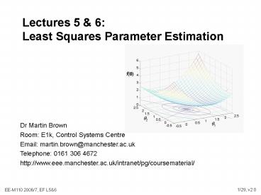
Lectures 5 6Least Squares Parameter Estimation
Dr Martin Brown Room E1k, Control Systems
Centre Email martin.brown_at_manchester.ac.uk Teleph
one 0161 306 4672 http//www.eee.manchester.ac.uk
/intranet/pg/coursematerial/
2
L56 Resources

• Core texts
• Ljung, Chapters 47
• Norton, Chapter 4
• On-line, Chapters 45
• In these two lectures, were looking at basic
  discrete time representations of linear, time
  invariant plants and models and seeing how their
  parameters can be estimated using the normal
  equations.
• The key example is the first order, linear,
  stable RC electrical circuit which we met last
  week, and which has an exponential response.

3
L56 Learning Objectives

• L5 Linear models and quadratic performance
  criterion
• ARX ARMAX discrete-time, linear systems
• Predictive models, regression and exemplar data
• Residual signal
• Performance criterion
• L6 Normal equations, interpretation and
  properties
• Quadratic cost functions
• Derive the normal equations for parameter
  estimation
• Examples
• Were not too concerned with system dynamics
  today, were concentrating on the general form of
  least squares parameter estimation

4
Introduction to Parametric System Identification

• In a full, physical, linear model, the models
  structure and coefficients can be determined from
  first principles
• In most cases, we have to estimate/tune the
  parameters because of an incomplete understanding
  about the full system (unknown drag, )
• We can use exemplar data (input/output examples),
  x(t), y(t), to estimate the unknown parameters
• Initially assume that the structure is known
  (unrealistic, but ), and all that remains to be
  estimated are the parameter values.

y(t)
Model q
u(t)

w(t)
y(t)
Plant q
e(t)
v(t)
5
Recursive Parameter Estimation Framework
Model q(t-1)
-


y(t)
u(t)
Controller
Plant q


w(t)
e(t)
v(t)

• where
• q, q(t-1) are the real and estimated parameter
  vectors, respectively.
• u(t) is the control input sequence
• y(t), y(t), are the real and estimated outputs,
  respectively
• e(t) is a white noise sequence (output/measurement
  noise)
• w(t) is the disturbances from measurable sources

6
Basic Assumptions in System Identification

• It is assumed that the unobservable disturbances
  can be aggregated and represented by a single
  additive noise e(t). There may also be input
  noise. Generally, it is assumed to be zero-mean,
  Gaussian
• The system is assumed to be linear with
  time-invariant parameters, so q is not
  time-varying. This is only approximately true
  within certain limits
• The input signal u(t) is assumed exactly known.
  Often there is noise associated with
  reading/measuring it
• The system noise e(t) is assumed to be
  uncorrelated with the input process u(t). This
  is unlikely to be true for instance to due
  feedback of y(t)
• The input signals need to be sufficiently
  exciting, they need to excite all relevant modes
  in the model for identification and testing

7
Discrete-Time Transfer Function Models

• On this course, were primarily concerned with
  discrete time signals and systems.
• Real-world physical, mechanical, electrical
  systems are continuous
• Consider the CT resistor-capacitor circuit
• So let q-1 denote the backward shift operator
  q-1y(t)y(t-1), then we have
• NB we can use the c2d() Matlab function to go
  from the continuous time (transfer function,
  state space) domain to the discrete time,
  z-domain.

8
Transfer Function/ARX DT LTI Model

• The previous model is an example of an
  AutoRegressive with eXogenous input), which can
  be expressed more generally as
• Some comments about the form of this model.
• The degree of the polynomials determines the
  complexity of the systems response and the
  number of parameters that have to be estimated.
  The roots of A(q) determine system stability
• a01, without loss of generality, so the model
  can be written as a predictive model y(t)
  y(t-1) u(t-1)
• b00, as it is assumed that an input cannot
  instantly affect the output, and so there must be
  at least a delay of one time instant between u
  y (assumes a fast enough sample time, relative to
  the system dynamics).
• Typically eN(0,s2) independent and identically
  distributed
• Close relationship between the q-shift and
  z-transform
• When n0, this produces a finite impulse response

9
Linear Regression

• The ARX systems prediction model can be
  expressed as
• Here the models parameters can be written as
• Treat the model as a deterministic system
• This is natural if the error term is considered
  to be insignificant or difficult to guess
• This denotes the model structure M (linear, time
  invariant, for example), and a particular model
  with a parameter value q, is M(q).
• This can be written as a linear regression
  structure
• where
• Parameter vector
• Input vector
• The term regression comes from the statistics
  literature and provides a powerful set of
  techniques for determining the parameters and
  interpretating the models. Need access to
  previous outputs y(t-1)

10
LTI DT ARMAX Model

• A more general discrete time, linear time
  invariant model also includes Moving Average
  terms on the error/residual signal
• Here, we describe the equation error term, e(t),
  as a moving average of white noise (non-iid
  measurement errors)
• Simple example
• y(t) 0.5y(t-1) 0.3y(t-2) 1.2u(t-1) -
  0.3u(t-2) 0.5e(t) 0.5e(t-1)
• This can be written as a pseudolinear regression

11
Exemplar Training Data

• To estimate the unknown parameters q, we need to
  collect some exemplar input-output data, and
  system identification is then a process of
  estimating the parameter values that best fit the
  data.
• The data is generated by a system of noisy ARX
  linear equations of the form
• where
• y is a column vector of measured plant outputs
  (T,1)
• X is a matrix of input regressors (T,nm)
• q is the true parameter vector (nm,1)
• e is the error vector (T,1)
• Each row of X represents a single input/output
  sample. Each column of X represents a time
  delayed output or input.
• Note that there is a burn-in period to measure
  the time-delayed outputs y(1), y(2), which are
  necessary to form the inputs to the time-delayed
  vector
• y(1), , y(t-n)

12
Example Data for 1st Order ARX Model

• 1st Order model representation
• First order plant model (exponential decay) with
  no external disturbances and the measurement
  noise is additive (Slide 7)
• Input vector, output signal and parameters
• At time t, the 1st order DT model is represented
  as
• Output y(t)
• Input x(t) y(t-1) u(t-1)
• Parameters q q1 q2
• Data
• As there are two parameters, if the system is
  truly first order and there is no measurement
  noise on any of the signals, we just need two
  (linearly independent) samples to estimate q.
• If there is measurement noise in y(t), we need to
  collect more data to reduce the effect of the
  random noise.
• Store Xy(1) u(1) y(2) u(2) y(3) u(3) ,
  yy(2) y(3) y(4)

13
Prediction Residual Signal

• The residual signal (measured-predicted) is
  defined as
• and can be represented as
• A simple regression interpretation is
• (each x represents an exemplar
• sample from a single input,
• single output system)

r(t)
residual
x(t)
Model q
-


y(t)
x(t)
output measurement
Plant q


e(t)
x
x
x
x
x
x
x
14
Measures of Model Goodness

• The models response can be expressed as
• y(t) xT(t)q
• where q is the models estimated parameter vector
  and x(t) is the input vector
• If y(t)y(t), the models response is correct for
  that single time sample. The residual
  r(t)y(t)-y(t) is zero. The residuals magnitude
  gives us an idea of the goodness of the
  parameter vector estimate for that data point.
• For a set of measured outputs and predictions
  y(t),y(t)t, the size of the residual vector
  ry-y, is an estimate of the parameter goodness
• We can determine the size by looking at the norm
  of r.

15
Residual Norm Measures

• A vector p-norm (of a vector r) is defined by
• The most common p-norm is the 2-norm
• The vector p-norm has the properties that
• r ? 0
• r 0 iff r 0
• kr kr
• r1r2 ? r1r2
• For the residual vector, the norm is only zero if
  all the residuals are zero. Otherwise, a small
  norm means that, on average, the individual
  residuals are small in magnitude.

16
Sum of Squared Residuals

• The most common discrete time performance index
  is the sum of squared residuals (2-norm squared)
• For each data point, the models output is
  compared against the plants and error is squared
  and summed over the remaining points.
• Any non-zero value for any of the residual values
  will mean that the performance index is positive
• The performance function f(q) is a function of
  the parameter values, because some parameter
  values will cause large residuals, others will
  cause small residuals.
• We want the parameter values that minimize f(q)
  (?0).

17
Relationship between Noise Residual

• The aim of parameter estimation is to estimate
  the values of q that minimize this performance
  index (sum squared residuals or errors SSE).
• When the model can predict the model exactly
• r(t) e(t)
• The residual signal is equal to the additive
  noise signal
• Note that the SSE is often replaced by the mean
  squared error MSE defined by
• MSE SSE/T ? s2 (the variance of the additive
  noise signal)
• This is the variance of the residual signal.
• This is simply represents the average squared
  error and ensures that the performance function
  does not depend on the amount of data
• Example, when we have 1000 repeated trials (step
  responses) of 9 data points for the DT electric
  circuit, with additive noise N(0,0.01)
• MSE r22/T 0.0103 ? s2
• RMSE 0.1015 ? s

18
Example DT RC Electrical Circuit

• Consider the DT, first order, LTI representation
  of the RC circuit which is an ARX model (Slide 7
  12)
• Assume that D/RC0.5, then
• y(t) 0.5y(t-1) 0.5u(t-1)
• Here the system is initially at rest y(0)0.
  Note that u here refers to a step signal which is
  switched on at t1 u(0)0, rather than the
  control signal
• Assume that 10 steps are taken, we collect 9 data
  points for system identification
• gtgt Xy(1end-1) u(1end-1)
• gtgt y1 y(2end)
• Gaussian random noise of standard error 0.05 was
  also added to y1
• gtgt y1e y10.05randn(size(y1))

19
Example Noisy Electric Circuit
NB randn(state, 123456)

• Note here, were cheating a bit by assuming the
  exact measurement y(t-1) is available to the
  models input but only the noisy measurement
  ye(t) is available to the models output.
• NB, in these notes, y() generally denotes the
  noisy output

20
Parameter Estimation

• An important part of system identification is
  being able to estimate the parameters of a linear
  model, when a quadratic performance function is
  used to measure the models goodness.
• This produces the well-known normal equations for
  least squares estimation
• This is a closed form solution
• Efficiently and robustly solved (in Matlab)
• Permits a statistical interpretation
• Can be solved recursively
• Investigated over the next 3-4 lectures

21
Noise-free Parameter Determination

• Parameter estimation works by assuming a
  plant/model structure, which is taken to be
  exactly known.
• If there are nm parameters in the model, we can
  collect nm pieces of data (linearly independent
  to ensure that the input/data matrix, X, is
  invertible)
• Xq y
• and invert the matrix to find the exact parameter
  values
• q X-1y
• In Matlab, both of the following forms are
  equivalent
• theta inv(X)y
• theta X\y
• theta 0.5 0.5 Previous example

22
Linear Model and Quadratic Performance

• When the model is linear and the data is noisy
  (missing inputs, unmeasurable disturbances), the
  Sum Squared Error (SSE) performance index can be
  expressed as
• This expression is quadratic in q. Typically
• size(X,1)gtgtsize(X,2)
• It is of the form (for 2 inputs/parameters)
• The equivalent system of linear equations Xqye
  is inconsistent

23
Quadratic Matrix Representation

• This can also be expressed in matrix form
• The general form for a quadratic is
• where

Hessian/covariance matrix
Cross-correlation vector
24
Normal Equations for a Linear Model

• When the parameter vector is optimal
• For a quadratic MSE with a linear model
• At optimality
• In Matlab, the normal equations are
• thetaHat inv(XX)Xy
• thetaHat pinv(X)y
• thetaHat X\y

25
Example 1 2 Parameter Model

• Data 3 data and 2 unknowns

Find Least Squares solution to
Form variance/covariance matrix and cross
correlation vector
Invert variance/covariance matrix
Least squares solution
26
Example 2 Electrical Circuit ARX Model
See slides 7, 12, 18 19

• 9 exemplars and 2 parameters. Additive
  measurement noise

Hessian (variance/covariance) matrix and
correlation vector
Inverse Hessian matrix
Least squares solution
NB randn(state, 123456)
27
Investigation into the Performance Function

• We can plot the performance index against
  different parameter values in a model
• As shown earlier, f() is a quadratic function in
  q
• It is centred at q, I.e. f(q) min f(q)
• The shape (contours) depends on the Hessian
  matrix X, this influences the ability to identify
  the plant. See next lectures

28
L56 Summary

• ARX and ARMAX discrete time linear models are
  widely used
• System identification is being considered simply
  as parameter estimation
• The residual vector is used to assess the quality
  of the model (parameter vector)
• The sum, squared error/residual (2-norm) is
  commonly used to measure the residuals size
  because it can be interpreted as the noise
  variance and because it is analytically
  convenient
• For a linear model, the SSE is a quadratic
  function of the parameters, which can be
  differentiated to estimate the optimal parameter
  via the normal equations

29
L56 Lab

• Theory
• Make sure you can derive the normal equations
  S22-24
• Matlab
• Implement the DT RC circuit simulation, S18, so
  you can perform a least squares parameter
  estimation given noisy data about the electrical
  circuit
• Set the Gaussian random seed, as per S26 and
  check your estimates are the same
• Set different seed and note that the optimal
  parameter values are different
• Perform the step experiment 10, 100, 1000,
  times and note that the estimated optimal
  parameter values tend towards the true values of
  0.5 0.5.
• Load the data into the identification toolbox GUI
  and create a first order parametric model with
  model orders 1 1 1. NB you do not need to
  remove the means from the data (why not?).
  Calculate the model and view the value of the
  parameters and the model fit, as well as checking
  the step response and validating the model.