March 19, 2003

1
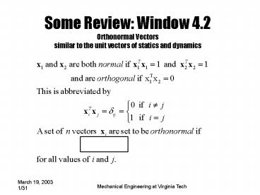
Some Review Window 4.2Orthonormal
Vectorssimilar to the unit vectors of statics
and dynamics
2
Ways of Normalizingthere are several methods of
fixing the magnitude of modes
1) Find the missing component by fixing it then
computing
2) Scaling with respect to the mass
3) Consider the transformation used here and
compute
3
4.3 - Modal Analysis

• Physical coordinates are not always the easiest
  to work in
• Eigenvectors provide a convenient transformation
  to modal coordinates
• Modal coordinates are linear combination of
  physical coordinates
• Say we have physical coordinates x and want to
  transform to some other coordinates u

4
Review of the Eigenvalue Problem
5
Eigenproblem (cont)

• Now we have a symmetric, real matrix
• Guaranteed real eigenvalues and distinct,
  mutually orthogonal eigenvectors

6
Eigenvectors Mode Shapes?
7
Eigenvectors vs. Mode Shapes
8
Eigenproblem (cont)

• Now we have decoupled the EOM i.e., we have n
  independent 2nd-order systems in modal
  coordinates r(t)

9
Decoupled EOM
(w1)2
k1
k2
(w2)2
Physical Co-ordinates. Coupled equations
Modal Co-ordinates. Uncoupled equations
Figure 4.5
10
Modal Transforms to SDOF

• The modal transformation
• transforms our 2 DOF to 2 SDOF systems
• This allows us to solve the two decoupled SDOF
  systems independently using the methods of
  chapter 1
• Then we can recombine using the inverse
  transformation to obtain the 2 DOF solution

11
Initial Conditions

• Must transform the initial conditions to modal
  coordinates
• Easy since we left a clear path

12
Free Response

• Calculate for each of the n equations
  independently

13
Response in Physical Coordinates

• With n DOFs and m time values

14
Example 4.3.1

• Follow steps in Window 4.4 (pg 272)

Kt Minv2KMinv2 Kt 3 -1 -1 3
Minv2 inv(sqrt(M)) Minv2 0.3333
0 0 1.0000
15
Example 4.3.1 (cont)
3) Calculate the symmetric eigenvalue problem
for K tilde P,D eig(Kt) lambda,Isort(diag(
D)) just sorts smallest to largest PP(,I)
reorder eigenvectors to match eigenvalues lambda
2 4 P -0.7071 -0.7071
-0.7071 0.7071
16
Example 4.3.1 (cont)
4) Calculate S M(-1/2) P and Sinv PT
M(1/2) S Minv2 P Sinv inv(S) 5)
Calculate the modal initial conditions r0 Sinv
x0 rdot0 Sinv v0
17
Example 4.3.1 (cont)
6) Find the free response in modal
coordinates tmax 10 numt 1000 t
linspace(0,tmax,numt) T,Wmeshgrid(t,lambda.(1
/2)) Use Tony's trick R0 r0(,ones(numt,1))
RDOT0 rdot0(,ones(numt,1)) r
RDOT0./W.sin(W.T) R0.cos(W.T) 7)
Transform back to physical space x Sr
18
Example 4.3.1 (cont)
Plot results figure subplot(2,1,1) plot(t,r(1,
),'-',t,r(2,),'--') title('free response in
modal coordinates') xlabel('time
(sec)') legend('r_1','r_2') subplot(2,1,2) plot(t
,x(1,),'-',t,x(2,),'--') title('free response
in physical coordinates') xlabel('time
(sec)') legend('x_1','x_2')
19
Modal and Physical Responses
Free response in modal coordinates
4
Modal Coordinates Independent oscillators
r
1
2
r
2
0
-2
-4
0
1
2
3
4
5
6
7
8
9
10
p sec
4.44 sec
Free response in physical coordinates
4
x
1
2
x
2
Physical Coordinates Coupled oscillators Note IC
0
-2
-4
0
1
2
3
4
5
6
7
8
9
10
Time (s)
20
Section 4.4 More then 2 Degrees of Freedom

• Extending previous section to any number of
  degrees of freedom

21
Many systems have large numbers of dof.
Just get more modal equations, one for
each degree of freedom (n is the number of dof)
22
Mode Summation Approach

• Based on the idea that any possible time response
  is just a linear combination of the eigenvectors

23
Mode Summation Approach (cont)
24
Mode Summation Approach (cont)
25
Mode Summation Approach (cont)
26
Mode Summation Approach (cont)

• Watch out for rigid-body modes!!

27
Example 4.3.1 by MSA
28
Example 4.3.1 by MSA (cont)
29
Alternate Path to Symmetric Single-Matrix
Eigenproblem

• Square root of matrix conceptually easy, but
  computationally expensive
• More efficient to decompose M into product of
  upper and lower triangular matrices (Cholesky
  decomposition)

30
Cholesky Decomposition
31
Cholesky (cont)

• Is this really faster? Lets ask MATLAB
• sqrtm requires a singular value decomposition
  (SVD), whereas Cholesky requires only simple
  operations

M 9 0 0 1 flops(0) sqrtm(M)
flops ans 65
M 9 0 0 1 flops(0) chol(M) flops ans
5