Recap: Other parameters and their sample statistics in H'T' Proportions

1
Recap Other parameters and their sample
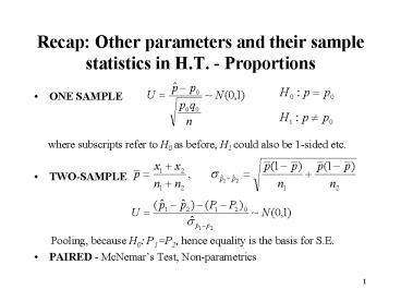
statistics in H.T. - Proportions

• ONE SAMPLE
• where subscripts refer to H0 as before, H1
  could also be 1-sided etc.
• TWO-SAMPLE
• Pooling, because H0 P1P2, hence equality
  is the basis for S.E.
• PAIRED - McNemars Test, Non-parametrics

2
Examples - 1-sample/2-sample H.T. on proportions

• In a survey of injecting drug users, 18 out of
  423 were HIV positive. Claim fewer than five
  percent in IDU population HIV positive?
• Hypothesised
  proportion 0.05 gives
• 
  while
• 1-sided at ? 0.01, has a U - 2.33, while
  from data
• 
  Clearly, test inconclusive at ? 0.01
• Two groups of patients, 55 with hypertension of
  whom 24 on special diet, 149 without, of whom 36
  on special diet. Can we say?
• 
  Test at 5 level of significance.
• From data, we have,
• 
  so Reject H0 at
  ?0.05

3
1-Sample/2-Sample Estimation/Testing for Variances

• Recall estimated sample variance
• Recall form of ?2 random variable
• Given in C.I. form, but H.T. complementary of
  course. Thus 2-sided
• H0 ?2 ?02 , ? ?2 from sample must be
  outside either limit to be in rejection region of
  H0

4
Variances - continued

• TWO-SAMPLE
• after manipulation - gives
• and where, conveniently
• BLOCKED - like paired for e.g. mean. Depends on
  Experimental Designs (ANOVA) used.

5
Examples on Estimation/H.T. for Variances

• Given a simple random sample, size 12, of animals
  studied to examine release of mediators in
  response to allergen inhalation. Known S.E. of
  sample mean 0.4 from subject measurement. Can
  we claim on the basis of data that population
  variance is not 4?
• From tables, critical values
  are 3.816 and 21.920 at 5 level, whereas the
  data give
• So cannot reject H0 at ?0.05
• Two different microscopic methods available.
  Repeated observations on standard object give
  estimates of variance
• 
  Test statistic
• where critical
  values for dof 9 and 28 3.52 for ?
• 0.02. Significant
  at 2-sided 2 level Reject H0

6
Many-Sample Tests - Counts/Frequencies
Chi-Square Goodness of Fit

• BasisTo test the hypothesis H0 that a set of
  observations is consistent with a given
  probability distribution (p.d.f.). For a set of
  categories, (distribution values), record the
  observed Oj and expected Ej number of
  observations that occur in each
• Under H0, Test Statistic
• distribution, where n is the number of
  categories.
• E.g. A test of expected segregation ratio is a
  test of this kind. So, for Backcross mating,
  expected counts for the 2 genotypic classes in
  progeny can be calculated using 0.5n, (B(n,
  0.5)). For F2 mating, expected counts two
  homozygous classes, one heterozygous class are
  0.25n,0.25n, 0.5n respectively. For F2 with
  segregants for dominant gene, dominant/recessive
  exp. counts 0.75n and 0.25n respectively.

7
Example.
Example. 40 dishes are counted to determine No.
organisms as follows. Aim to test at the 0.05
level of significance if the results are
consistent with hypothesis that outcomes across
cultures randomly distributed. No.
organisms 1-25 26 - 50 51 - 75
76 - 100 Total Observed No. dishes 6
12 14 8
40 Expected No. dishes 10 10
10 10 40Test
statistic (6-10)2/10 (12-10)2/10
(14-10)2/10 (8-10)2/10 4. The 0.05
critical value of c 23 7.81, so the test is
inconclusive.Note In general the chi square
tests tend to be very conservative vis-a-vis
other tests of hypothesis, (i.e. tend to give
inconclusive results).
8
Chi-Square Contingency Test

• To test two random variables are statistically
  independent
• Under H0, Expected number of observations for
  cell in row i and column j is the appropriate row
  total ? the column total divided by the grand
  total. The test statistic for table n rows, m
  columns
• D.o.f.
• Simply - the chi-square distribution is the sum
  of k squares of independent random variables,
  i.e. defined in a k-dimensional space.
• Constraints, e.g. forcing sum of observed and
  expected observations in a row or column to be
  equal, or e.g. estimating a parameter of the
  parent distribution from sample values, reduce
  dimensionality of the space by 1 each time, e.g.
  contingency table, with m rows, n columns has Em
  , En predetermined, so d.o.f.of the test
  statistic is (m-1) (n-1).

9
Example

• In the following table, the figures in brackets
  are expected values.
• Results Method 1 Method 2
  Method 3 Totals
• High 100 (50) 70 (67)
  30 (83) 200
• Medium 130 (225) 320 (300) 450
  (375) 900
• Low 70 (25) 10 (33)
  20 (42) 100
• Totals 300 400 500
  1200
• T.S. (100-50)2/ 50 (70 - 67)2/ 67
  (30-83)2/ 83 (130-225)2/225 (320-300)2/ 300
  (450-375)2/375 (70-25)2/ 25 (10-33)2/ 33
  (20-42)2/ 42 248.976
• The 0 .05 critical value for c 22 ? 2 is 9.49 so
  H0 rejected at the .05 level of significance.

10
?2- Extensions

• Example Recall Mendels data, (Lectures Week 3).
  The situation is one of multiple populations,
  i.e. round and wrinkled. Then
• where subscript i indicates population, m is the
  total number of populations and n No. plants, so
  calculate ?2 for each cross and sum.
• Pooled ?2 estimated using marginal frequencies
  under assumption same S.R. all 10 plants

11
?2 -Extensions - contd.

• So, a typical ?2-Table for a single-locus
  segregation analysis, for n No. genotypic
  classes and m No. populations.
• Source dof Chi-square
• Total nm-1 ?2Total
• Pooled n-1 ?2Pooled
• Heterogeneity n(m-1) ?2Total -?2Pooled
• Thus for the Mendel experiment, testing separate
  null hypotheses
• (1) A single gene controls the seed character
• (2) The F1 seed is round and heterozygous (Aa)
• (3) Seeds with genotype aa are wrinkled
• (4) The A allele (normal) is dominant to a allele
  (wrinkled)

12
Analysis of Variance/Experimental Design-Many
samples, Means and Variances

• Analysis of Variance (AOVor ANOVA) was
• originally devised for agricultural
  statistics
• on e.g. crop yields. Typically, row and
  column format, small plots of a fixed size.
  The yield
• yi, j within each plot was recorded. One
  Way classificationModel yi, j i
  i, j , i ,j -gt N (0, s)where
  overall mean
  i effect of the ith factor i, j error
  term.Hypothesis H0 1 2
  m

y1, 3
y1, 1
y1, 2
y1, 4
y1, 5
1
y2, 2
y2, 1
y2, 3
2
y3, 1
y3, 2
y3, 3
3

13
Totals MeansFactor
1 y1, 1 y1, 2 y1, 3 y1, n1
T1 y1, j y1. T1 / n1
2 y2, 1 y2,, 2 y2, 3 y1, n2 T2
y2, j y2. T2 / n2
m ym, 1 ym, 2 ym, 3 ym, nm
Tm ym, j ym. Tm / nmOverall mean
y yi, j / n, where n
niDecomposition (Partition) of Sums of
Squares (yi, j - y )2
ni (yi . - y )2 (yi, j - yi .
)2 Total Variation (Q) Between Factors (Q1)
Residual Variation (QE )Under H0 Q /
(n-1) -gt 2n - 1, Q1 / (m - 1) -gt
2m - 1, QE / (n - m) -gt 2n - m
Q1 / ( m - 1 )
-gt Fm - 1, n - m QE / ( n - m ) AOV
Table Variation D.F. Sums of
Squares Mean Squares F
Between m -1 Q1 ni(yi. - y
)2 MS1 Q1/(m - 1) MS1/ MSE
Residual n - m QE (yi, j -
yi .)2 MSE QE/(n - m) Total
n -1 Q (yi, j. - y )2
Q /( n - 1)
14
Two-Way Classification
Factor I MeansFactor II y1, 1 y1, 2
y1, 3 y1, n y1.

. ym, 1 ym, 2
ym, 3 ym, n ym.
Means y. 1 y. 2 y. 3
y . n y . . Write as y
Partition SSQ (yi, j - y )2
n (yi . - y )2 m (y . j - y )2
(yi, j - yi . - y . j y )2
Total Between
Between Residual
Variation Rows
Columns VariationModel yi, j
i j i, j
, i, j -gt N ( 0, s)H0 All i are equal
and all j are equalAOV Table Variation
D.F. Sums of Squares Mean
Squares F Between m -1
Q1 n (yi . - y )2 MS1
Q1/(m - 1) MS1/ MSE Rows
Between n -1 Q2 m (y. j - y )2
MS2 Q2/(n - 1) MS2/ MSE
Columns Residual
(m-1)(n-1) QE (yi, j - yi . - y. j y)2
MSE QE/(m-1)(n-1) Total mn
-1 Q (yi, j. - y )2
Q /( mn - 1)
15
Two-Way Example
Factor I 1 2 3 4
5 Totals Means Variation d.f. S.S.
F Fact II 1 20 18 21
23 20 102 20.4 Rows
3 76.95 18.86 2 19 18
17 18 18 90 18.0
Columns 4 8.50 1.57 3 23
21 22 23 20 109
21.8 Residual 12 16.30 4 17
16 18 16 17 84
16.8 Totals 79 73 78
80 75 385 Total 19
101.75 Means 19.75 18.25 19.50 20.00
18.75 19.25FYI software such as SPSS
is designed for analysing data that is recorded
with variables in columns and individual
observations in the rows. Thus the AOV data above
would be written as a set of columns or rows,
e.g. Variable 20 18 21 23 20 19 18 17
18 18 23 21 22 23 20 17 16 18 16
17Factor 1 1 1 1 1 1 2
2 2 2 2 3 3 3 3 3 4
4 4 4 4Factor 2 1 2 3 4
1 2 3 4 1 2 3 4 1 2
3 4 1 2 3 4