Quality of embeddings

1
Quality of embeddings

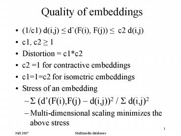
• (1/c1) d(i,j) d(F(i), F(j)) c2 d(i,j)
• c1, c2 1
• Distortion c1c2
• c2 1 for contractive embeddings
• c11c2 for isometric embeddings
• Stress of an embedding
• S (d(F(i),F(j) d(i,j))2 / S d(i,j)2
• Multi-dimensional scaling minimizes the above
  stress

2
Multi-Dimensional Scaling

• Map the items in a k-dimensional space trying to
  minimize the stress
• Steepest Descent algorithm
• Start with an assignment
• Minimize stress by moving points
• Can be computationally expensive

3
Dimensionality reduction

• DFT
• Wavelets
• Space-filling curves
• Fastmap
• SVD
• Embedding of metric spaces
• Random projections

4
Space-filling curves

• Basic assumption Finite precision in the
  representation of each co-ordinate, K bits (2K
  values)
• The address space is a square (image) and
  represented as a 2K x 2K array
• Each element is called a pixel
• Impose a linear ordering on the pixels of the
  image
• Column-wise scan
• Z-order
• Hilbert order
• Generalize to multiple dimensions

5
Z-ordering

• Given a point (x, y), find the pixel for the
  point and then compute the z-value

A
ZA shuffle(xA, yA) shuffle(01, 11)
11
0111 (7)10
10
ZB shuffle(01, 01) 0011
01
00
contractive? c1? c2?
00
01
10
11
B
Generalize to higher dimensions
6
Queries

• Find the z-values that are contained in the query
  and then find the enclosing ranges

QA
QA ? range 4, 7
11
QB ? ranges 2,3 and 8,9
10
01
00
00
01
10
11
QB
7
Hilbert curve

• We want points that are close in 2d to be close
  in the 1d
• Note that in 2d there are 4 neighbors for each
  point whereas in 1d there are only 2.
• Z-curve has some jumps that we would like to
  avoid
• Hilbert curve avoids the jumps recursive
  definition

8
Hilbert Curve- example

• It has been shown that in general Hilbert is
  better than the other space filling curves for
  retrieval Jag90
• Hi (order-i) Hilbert curve for 2ix2i array

H1
...
H(n1)
H2
9
References

• Linear clustering of objects with multiple
  attributes, H.V. Jagadish, SIGMOD 1990
• Analysis of the Clustering Properties of the
  Hilbert Space-Filling Curve, B. Moon, H.V.
  Jagadish,C. Faloutsos, and J.H. Saltz, IEEE
  Knowledge and Data Engineering, 13(1), 124-141,
  2001.

10
Dimensionality reduction

• DFT
• Wavelets
• Space-filling curves
• Fastmap
• SVD
• Embedding of metric spaces
• Random projections

11
FastMap

• Embedding of a metric space (X,d) into a vector
  space.
• Faloutsos and Lin (1995) proposed FastMap as
  metric analogue to the KL-transform (PCA).
  Imagine that the points are in a Euclidean space.
• Select two pivot points xa and xb that are far
  apart.
• Compute a pseudo-projection of the remaining
  points along the line xaxb . This results in
  the first coordinate for all the points.
• Project the points to an orthogonal subspace
  and recurse.

12
Selecting the Pivot Points

• The pivot points should lie along the principal
  axes, and hence should be far apart.
• Select any point x0.
• Let x1 be the farthest from x0.
• Let x2 be the farthest from x1.
• Return (x1, x2).

x2
x0
x1
13
Pseudo-Projections

• Given pivots (xa , xb ), for any third point y,
  we use the law of cosines to determine the
  projection of y along xaxb .
• The pseudo-projection for y is
• This is first coordinate.

xb
db,y
da,b
y
cy
da,y
xa
14
Project to orthogonal plane
xb
cz-cy

• Given distances along xaxb we can compute
  distances within the orthogonal hyperplane
  using the Pythagorean theorem.
• Using d (.,.), recurse until k features chosen.

z
dy,z
y
xa
y
z
dy,z
15
Example
16
Example

• Pivot Objects O1 and O4
• X1 O10, O20.005, O30.005, O4100, O599
• For the second iteration pivots are O2 and O5

17
Experiments

• Stress and response time (embedding)
• WINE dataset
• Euclidean distance after attribute normalization
• Time versus database size
• Time versus number of dimensions
• Time versus stress (varying dimensions)
• Clustering
• Document dataset
• distance defined by transforming documents to
  vector space
• Gaussian (synthetic) dataset
• Euclidean distance after attribute normalization
• Spiral (synthetic) dataset
• Euclidean distance

18
FastMap problems

• If the original space is not a Euclidean space,
  then the projected distance may be a complex
  number!
• Not a contractive mapping for non-Euclidean spaces

19
References

• C. Faloutsos and K.-I. Lin, FastMap A Fast
  Algorithm for Indexing, Data-Mining and
  Visualization of Traditional and Multimedia
  Datasets, Proc. ACM SIGMOD, 1995, 163-174.
• G. Hjaltson and H. Samet, Properties of
  Embedding Methods for Similarity Searching in
  Metric Spaces, IEEE Transactions on Pattern
  Analysis and Machine Intelligence, May 2003,
  530-549. (Read sections 1, 2, 3.1, 4, 5)