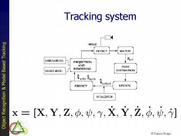
Tracking system

1
Tracking system
2
Motivation

• Manipulating objects in domestic environments
• Localization / Navigation
• Object Recognition
• Servoing Tracking
• Grasping Pose estimation

3
Steps

• Recognition (2D)
• Tracking (2D)
• Pose estimation (3D)
• Initial pose estimation

Where in the image ?
Where in the world ?
4
Initial Pose Estimation

• Recognition/Tracking Pose estimation
• (x,y) (X,Y,Z, f,
  y, g)

5
Example Objects
6
Characteristics

• Simple geometry (polyhedra, cones, cylinders)
• Specular surfaces
• Background
• Illumination
• Slippery objects

7
Characteristics

• Simple geometry wireframe models
• Specular surfaces - ll
• Illumination - ll
• Background - ll
• Highly texture appearance
• Slippery objects power grasps

8
Model Based Techniques

• Appearance based methods
• Geometry based methods
• 3D wireframe models
• Complete pose estimation
• Techniques from computer graphics used for
  rendering

FUSION!
9
Object Recognition

• Removes background, preserves object.
• Necessary to raise the signal to noise ratio, for
  the pose estimatior.
• Solved using color cooccurrence histograms.

10
Pose Estimation

• An apperance based method is used to recognize
  the object, and estimate an initial pose.
• A geometric model based method is used to obtain
  an accurate pose.
• Algorithm combines the robustness of appearance
  based methods with the accuracy of feature based
  methods.

11
(No Transcript)
12
(No Transcript)
13
Color Cooccurrence Histograms

• Apperance based method.
• Based on color cues only.
• Superior to standard color histograms.
• Invariant to translation and rotation.
• Robust towards scale changes.

14
Building Color Cooccurrence Histograms

• All pairs of pixels within a certain radius
  contribute to the histogram.
• Example 4x4 image with 3 colors, and a maximum
  radius of 3 pixels.

Histogram
15
Building Color Cooccurrence Histograms

• When all pairs have been counted, the histogram
  is normalized. Each bin is divided with the total
  number of pixel pairs.

50
Histogram
16
Color Cooccurrence Histograms - Matching

• A common histogram matching method is used.

• Reduces the effect of background noise, as
  unexpected colors will not penalize the match
  value.

17
Color Quantization

• Before the histogram can be built, the colors in
  the image need to be quantized. This is done
  using k-means clustering.

Red
Green
18
Color Quantization

• Images are normalized prior to quantization, in
  order to decrease the effect of varying lighting
  conditions.
• Only the red and green components are preserved.
• Performance equal to RGB and HSV.

Red
Green
19
Color Constancy Problem

• If lighting conditions change, colors may fall
  out of their original cluster, or even worse,
  into another one.

Red
green light
Green
20
Object Segmentation - Training

• The system was trained using both front and back
  sides of the objects.
• The background of the training images was
  manually removed before training.

21
Object Segmentation

• A search window scans through the image,
  comparing the cooccurrence histogram with the
  stored histogram from the training images. The
  result is a vote matrix.

22
Object Segmentation

• From the vote matrix, segmentation windows are
  contructed.
• Starting from the global maximum, adjacent rows
  and columns are added as long as the vote values
  give sufficient support.

23
Object Segmentation - Results

• Out of 50 test images, 49 objects were
  successfully segmented.
• Average segmentation time was 1.7 s on a 500 MHz
  Sun station.

24
Pose Estimation

• The geometric model based pose estimator requires
  an initial pose to converge. The initial pose is
  estimated using color cooccurrence histograms.

25
Pose Estimation - Training

• 70 training images were used.
• The pose of the object varied over the training
  images.
• The correct pose of the object in the training
  image was stored, together with the cooccurrence
  histogram.

26
Pose Estimation

• The object with the unknown pose is compared to
  each of the training examples. The result is a
  match value graph.

27
Pose Estimation

• The match value graph is filtered using a
  Gaussian kernel.
• Superior method compared to a nearest-neighbor
  approach.

28
Initial Pose Estimation

• Appearance based

29
Principle Component Analisys

• Learning stage compressing image set using
  eigenspace representation PCA PCA
• Pose recognition stage closest point search on
  appearance manifold PCA
• Fitting stage closest line search for pose
  refinement

30
PCA i(q)

• Pose
• Appearance
• Eigenstructure
  decomposition
  problem
• PCA

31
PCA

• Implicit covariance matrix
  (conjugate gradient
  method)
• PCA

32
PCA

• Pose determination
• PCA

33
Initialization by PCA
34
Geometric Model Based Pose Estimation

• Finally, the algorithm was integrated with the
  model based pose estimator.

35
Geometric Model Based Pose Estimation
36
Local refinement by tracking

• H (14 0 60 15 6 5) mm, deg

37
Modeling
38
Modeling
39
Pose estimation

• DeMenthon and Davis 1995
• Orthographic projection
• Iterative method
• No initial guess needed
• This step is followed by an extension of Lowes
  nonlinear approach
• (Canceroni, Araujo and Brown et al.)

40
Tracking

• Lie algebra approach
• Rigid body motion SE(3) (6D Lie group)
• 
  

41
Image motion

• with
• L - observed motion in an image point

i
42
Normal flow
43
Rendering example
44
3D pose update

• The change in pose is estimated using least
  square approach
• where a represents the quantities of Euclidian
  motion

i
45
3D pose update
46
Examples
47
Examples
48
Example
49
Task 1 Align and Track
50
Task 1 Align and Track
51
Task 2 Object Positioning
52
(No Transcript)
53
(No Transcript)
54
Task 3 - Insertion
55
Insertion task

• How much
• a-priori info
• can we used?

56
Pick and Place