
Operational Environmental Prediction: Nearshore Water Quality in the Great Lakes PowerPoint PPT Presentation
1 / 27
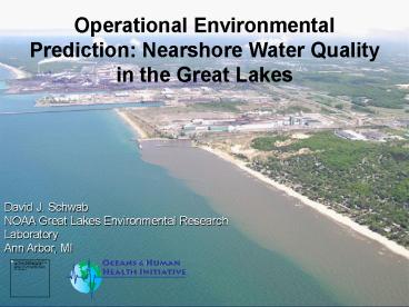
Title: Operational Environmental Prediction: Nearshore Water Quality in the Great Lakes
1
Operational Environmental Prediction Nearshore
Water Quality in the Great Lakes
David J. Schwab NOAA Great Lakes Environmental
Research Laboratory Ann Arbor, MI
2
Factors Contributing to Nearshore Water Quality
in the Great Lakes
Climate Meteorology Hydrology Hydrodynamics
Biology/Chemistry
3
Beach Closings or HABs
Meteorology
Meteorology
Change in Land-use
Change in Land-use
Change in Land-use
Hydrology/Water Flow Bacterial Fate
Hydrology/Water Flow Bacterial Fate
Beach Closings
Circulation and Bacterial Fate
Circulation and Bacterial Fate
4
- Outline
- Lake Michigan tributary modeling using
nested-grid hydrodynamic models - application to
beach water quality forecasting - Lake Erie coupled physical/biological model -
application to HAB and hypoxia forecasting
5
Beach Closures
- Major health risk of microbial contamination by
bacteria, viruses and protozoa in recreational
waters - E.Coli requires a 24 hour incubation period
- People may unintentionally swim in contaminated
water
6
(No Transcript)
7
Lake Michigan Beach Quality Forecasting
Lakewide grid (POM model)
Coupled models nested grids
Burns Ditch nested model grid
8
Princeton Ocean Model (Blumberg and Mellor,
1987) - Fully three-dimensional nonlinear
Navier-Stokes equations - Flux form of
equations - Boussinesq and hydrostatic
approximations - Free upper surface with
barotropic (external) mode - Baroclinic
(internal) mode - Turbulence model for vertical
mixing - Terrain following vertical coordinate
(ltsigmagt-coordinate) - Generalized orthogonal
horizontal coordinates - Smagorinsky horizontal
diffusion - Leapfrog (centered in space and time)
time step - Implicit scheme for vertical mixing -
Arakawa-C staggered grid - Fortran code optimized
for vectorization Application to the Great
Lakes - No open boundary - No tides - Uniform
salinity - Seasonal thermal structure - Uniform
rectangular grid - XDR used for input and output
- Nested grid considerations
- 3d boundary condition for u, v, and T
interpolated from coarse grid at each boundary
point - Vertically integrated velocity is specified for
external mode - Internal mode velocity and temperature are
specified from 3-d boundary condition for inflow,
use radiation condition for outflow - Water level is adjusted to maintain zero mean in
nested grid subdomain
9
Nested grid hydrodynamic models in Lake Michigan
10
Burns Ditch 100m computational grid
24 km
6 km
11
Web site www.glerl.noaa.gov/res/glcfs/bd
12
(No Transcript)
13
(No Transcript)
14
(No Transcript)
15
(No Transcript)
16
Great Lakes Coastal Forecasting System -
Operational Nowcast 20 day sample using
vertically averaged currents
17
- Lake Erie Coupled Physical/Biological model
18
The Problem - Excessive nutrient loading in the
1960s led to massive algal blooms, oxygen
depletion, and diminished water quality in Lake
Erie. - 1972 Water Quality Agreement between the
US and Canada limited P loads from municipal,
industrial, and agricultural sources. - With
controls, P levels decreased to acceptable levels
and water quality improved. - In recent years, P
levels in Lake Erie appear to be increasing,
despite controls.
19
The Problem - Excessive nutrient loading in the
1960s led to massive algal blooms, oxygen
depletion, and diminished water quality in Lake
Erie. - 1972 Water Quality Agreement between the
US and Canada limited P loads from municipal,
industrial, and agricultural sources. - With
controls, P levels decreased to acceptable levels
and water quality improved. - In recent years, P
levels in Lake Erie appear to be increasing,
despite controls.
Our Approach - Incorporate phosphorus transport
and fate dynamics into high resolution (hourly
time scale, 2 km horizontal resolution)
hydrodynamic model of Lake Erie as a first step
toward spatially explicit model of entire lower
food web
20
Lake Erie Physical Characteristics Surface
Area 25800 km2 Throughflow 6000
m3s-1 Volume 480 km3 Retention time 2.5
yrs Mean Depth 18.6 m
21
Ecosystem Forecasting of Lake Erie Hypoxia
- What are the Causes, Consequences, and Potential
Remedies of Lake Erie Hypoxia? - Linked set of models to forecast
- changes in nutrient loads to Lake Erie
- responses of central basin hypoxia to multiple
stressors - P loads, hydrometeorology, dreissenids
- potential ecological responses to changes in
hypoxia - Approach
- Models with range of complexity
- Consider both anthropogenic and natural stressors
- Use available data IFYLE, LETS, etc.
- Will assess uncertainties in both drivers and
models - Apply models within an Integrated Assessment
framework to inform decision making for policy
and management
22
Hypoxia Forecasting Modeling Approach
- Model ranging in complexity
- Correlation-based models
- 1D hydrodynamics with simple mechanistic WQ model
- Vertical profiles extracted from full
hydrodynamic model - TP, Carbon, Solids
- 3D hydrodynamics with simple mechanistic WQ model
- Physics from full hydrodynamic model
- 3D hydrodynamics with complex mechanistic WQ
model - WQ framework similar to Chesapeake Bay ICM model
- Multi-class phyto- and zooplankton, organic and
inorganic nutrients, sediment digenesis, etc - Addition of zebra mussels and other improvements
23
Chapra, S.C. 1980. J. Great Lakes Res.
6(2)101-112.
24
Effect of Phosphorus Controls on Lake Erie
Central Basin Springtime P Concentration (Ryan et
al., 1999)
25
(No Transcript)
26
Lake Erie 1994 physical/biological model
- Hydrodynamics
- - Great Lakes version of POM
- 20 vertical levels, 2 km horizontal grid (6500
cells) - Hourly meteorology (1994, JD 1-365)
- Realistic tributary flows
- Accounts for ice cover
- Mass balance for P
- POM hydrodynamics (2d for now)
- Realistic P loading
- Constant settling velocity (for now)
27
- Computer animation of model results
- Starts in January, 1994
- Uses 2d currents from hydrodynamic model
- Time dependent P loads
- Combination Lax-Wendroff and upwind advection
scheme - No horizontal diffusion
- Initial condition C 10 ug/L
- Settling velocity 6.8E-7 m/s (21 m/yr)
28
Questions?
Recommended
