Hebb Rule

1
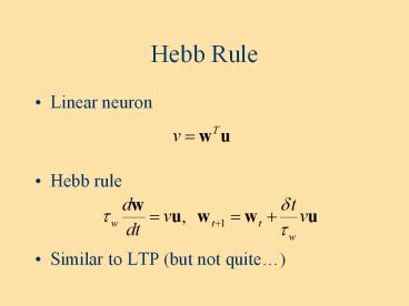
Hebb Rule

• Linear neuron
• Hebb rule
• Similar to LTP (but not quite)

2
Hebb Rule

• Average Hebb rule correlation rule
• Q correlation matrix of u

3
Hebb Rule

• Hebb rule with threshold covariance rule
• C covariance matrix of u
• Note that lt(v-lt v gt)(u-lt u gt)gt would be
  unrealistic because it predicts LTP when both u
  and v are low

4
Hebb Rule

• Main problem with Hebb rule its unstable Two
  solutions
• Bounded weights
• Normalization of either the activity of the
  postsynaptic cells or the weights.

5
BCM rule

• Hebb rule with sliding threshold
• BCM rule implements competition because when a
  synaptic weight grows, it raises by v2, making
  more difficult for other weights to grow.

6
Weight Normalization

• Subtractive Normalization

7
Weight Normalization

• Multiplicative Normalization
• Norm of the weights converge to 1/a

8
Hebb Rule

• Convergence properties
• Use an eigenvector decomposition
• where em are the eigenvectors of Q

9
Hebb Rule
e2
e1
l1gtl2
10
Hebb Rule
Equations decouple because em are the
eigenvectors of Q
11
Hebb Rule
12
Hebb Rule

• The weights line up with first eigenvector and
  the postsynaptic activity, v, converges toward
  the projection of u onto the first eigenvector
  (unstable PCA)

13
Hebb Rule

• Non zero mean distribution correlation vs
  covariance

14
Hebb Rule

• Limiting weights growth affects the final state

First eigenvector 1,-1
0.8
x
a
m
w
/
2
w
w
w
/
max
1
15
Hebb Rule

• Normalization also affects the final state.
• Ex multiplicative normalization. In this case,
  Hebb rule extracts the first eigenvector but
  keeps the norm constant (stable PCA).

16
Hebb Rule

• Normalization also affects the final state.
• Ex subtractive normalization.

17
Hebb Rule
18
Hebb Rule

• The constrain does not affect the other
  eigenvector
• The weights converge to the second eigenvector
  (the weights need to be bounded to guarantee
  stability)

19
Ocular Dominance Column

• One unit with one input from right and left eyes

s same eye
d different eyes
20
Ocular Dominance Column

• The eigenvectors are

21
Ocular Dominance Column

• Since qd is likely to be positive, qsqdgtqs-qd.
  As a result, the weights will converge toward the
  first eigenvector which mixes the right and left
  eye equally. No ocular dominance...

22
Ocular Dominance Column

• To get ocular dominance we need subtractive
  normalization.

23
Ocular Dominance Column

• Note that the weights will be proportional to e2
  or e2 (i.e. the right and left eye are equally
  likely to dominate at the end). Which one wins
  depends on the initial conditions.

24
Ocular Dominance Column

• Ocular dominance column network with multiple
  output units and lateral connections.

25
Ocular Dominance Column

• Simplified model

26
Ocular Dominance Column

• If we use subtractive normalization and no
  lateral connections, were back to the one cell
  case. Ocular dominance is determined by initial
  weights, i.e., it is purely stochastic. This is
  not whats observed in V1.
• Lateral weights could help by making sure that
  neighboring cells have similar ocular dominance.

27
Ocular Dominance Column

• Lateral weights are equivalent to feedforward
  weights

28
Ocular Dominance Column

• Lateral weights are equivalent to feedforward
  weights

29
Ocular Dominance Column
30
Ocular Dominance Column

• We first project the weight vectors of each
  cortical unit (wiR,wiL) onto the eigenvectors of
  Q.

31
Ocular Dominance Column

• There are two eigenvectors, w and w-, with
  eigenvalues qsqd and qs-qd

32
Ocular Dominance Column
33
Ocular Dominance Column

• Ocular dominance column network with multiple
  output units and lateral connections.

34
Ocular Dominance Column

• Once again we use a subtractive normalization,
  which holds w constant. Consequently, the
  equation for w- is the only one we need to worry
  about.

35
Ocular Dominance Column

• If the lateral weights are translation invariant,
  Kw- is a convolution. This is easier to solve in
  the Fourier domain.

36
Ocular Dominance Column

• The sine function with the highest Fourier
  coefficient (i.e. the fundamental) growth the
  fastest.

37
Ocular Dominance Column

• In other words, the eigenvectors of K are sine
  functions and the eigenvalues are the Fourier
  coefficients for K.

38
Ocular Dominance Column

• The dynamics is dominated by the sine function
  with the highest Fourier coefficients, i.e., the
  fundamental of K(x) (note that w- is not
  normalized along the x dimension).
• This results is an alternation of right and left
  columns with a periodicity corresponding to the
  frequency of the fundamental of K(x).

39
Ocular Dominance Column

• If K is a Gaussian kernel, the fundamental is the
  DC term and w ends up being constant, i.e., no
  ocular dominance columns (one of the eyes
  dominate all the cells).
• If K is a mexican hat kernel, w will show ocular
  dominance column with the same frequency as the
  fundamental of K.
• Not that intuitive anymore

40
Ocular Dominance Column

• Simplified model

41
Ocular Dominance Column

• Simplified model weights matrices for right and
  left eyes

W
W
W
- W