
Dynamic Light Scattering - PowerPoint PPT Presentation
1 / 52
Title:
Dynamic Light Scattering
Description:
Dynamic Light Scattering ZetaPALS w/ 90Plus particle size analyzer Also equipped w/ BI-FOQELS & Otsuka DLS-700 (Rm CCR230) Dynamic Light Scattering (DLS) Photon ... – PowerPoint PPT presentation
Number of Views:330
Avg rating:3.0/5.0
Title: Dynamic Light Scattering
1
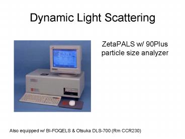
Dynamic Light Scattering
- ZetaPALS w/ 90Plus particle size analyzer
Also equipped w/ BI-FOQELS Otsuka DLS-700 (Rm
CCR230)
2
- Dynamic Light Scattering (DLS)
- Photon Correlation Spectroscopy (PCS)
- Quasi-Elastic Light Scattering (QELS)
- Measure Brownian motion by
- Collect scattered light from suspended particles
to - Obtain diffusion rate to
- Calculate particle size
3
Brownian motion
- Velocity of the Brownian motion is defined by the
Translational Diffusion Coefficient (D) - Brownian motion is indirectly proportional to
size - Larger particles diffuse slower than smaller
particles - Temperature and viscosity must be known
- Temperature stability is necessary
- Convection currents induce particle movement that
interferes with size determination - Temperature is proportional to diffusion rate
- Increasing temperature increases Brownian motion
4
Brownian motion
- Random movement of particles due to bombardment
of solvent molecules
5
Stokes-Einstein Equation
- dH hydrodynamic diameter (m)
- k Boltzmann constant (J/Kkgm2/s2K)
- T temperature (K)
- ? solvent viscosity (kg/ms)
- D diffusion coefficient (m2/s)
6
Hydrodynamic diameter
Particle diameter
- The diameter measured by DLS correlates to the
effective particle movement within a liquid - Particle diameter electrical double layer
- Affected by surface bound species which slows
diffusion
Hydrodynamic diameter
7
Nonspherical particles
Rapid
Equivalent sphere
Slow
Hydrodynamic diameter is calculated based on the
equivalent sphere with the same diffusion
coefficient
8
Experimental DLS
- Measure the Brownian motion of particles and
calculate size - DLS measures the intensity fluctuations of
scattered light arising from Brownian motion - How do these fluctuations in scattered light
intensity arise?
9
What causes light scattering from (small)
particles?
- Explained by JW Strutt (Lord Rayleigh)
- Electromagnetic wave (light) induces oscillations
of electrons in a particle - This interaction causes a deviation in the light
path through an angle calculated using vector
analysis - Scattering coefficient varies inversely with the
fourth power of the wavelength
10
Interaction of light with matterRayleigh
approximation
- For small particles (d ?/10), scattering is
isotropic - Rayleigh approximation tells us that
- I a d6
- I a 1/?4
- where I intensity of scattered light
- d particle diameter
- ? laser wavelength
11
Mie scattering from large particles
- Used for particles where d ?0
- Complete analytical solution of Maxwells
equations for scattering of electromagnetic
radiation from spherical particles - Assumes homogeneous, isotropic and optically
linear material
Stratton, A. Electromagnetic theory, McGraw-Hill,
New York (1941) www.lightscattering.de/MieCalc
12
Brownian motion and scattering
Constructive interference
Destructive interference
13
Brownian motion and scattering Multiple particles
14
Instrument layout
15
Intensity fluctuations
- Apply the autocorrelation function to determine
diffusion coefficient - Large particles smooth curve
- Small particles noisy curve
16
Determining particle size
- Determine autocorrelation function
- Fit measured function to G(t) to calculate G
- Calculate D, given n, ?, and G
- Calculate dH, given T and ?
User defined values.
17
How a correlator works
- Random motion of small particles in a liquid
gives rise to fluctuations in the time intensity
of the scattered light - Fluctuating signal is processed by forming the
autocorrelation function - Calculates diffusion
18
How a correlator works
- Large particles the signal will be changing
slowly and the correlation will persist for a
long time - Small, rapidly moving particles the correlation
will disappear quickly
19
The correlation function
- For monodisperse particles the correlation
function is - Where
- A baseline of the correlation function
- Bintercept of the correlation function
- G Dq2
- Dtranslational diffusion coefficient
- q(4pn/?0)sin(?/2)
- nrefractive index of solution
- ?0wavelength of laser
- ?scattering angle
20
The correlation function
- For polydisperse particles the correlation
function becomes - where g1(t) is the sum of all exponential decays
contained in the correlation function
21
Broad particle size distribution
- Correlation function becomes nontrivial
- Measurement noise, baseline drifts, and dust make
the function difficult to solve accurately - Cumulants analysis
- Convert exponential to Taylor series
- First two cumulants are used to describe data
- G Dq2
- µ2 (D2-D2)q4
- Polydispersity µ2/ G2
22
Cumulants analysis
- The decay in the correlation function is
exponential - Simplest way to obtain size is to use cumulants
analysis1 - A 3rd order fit to a semi-log plot of the
correlation function - If the distribution is polydisperse, the semi-log
plot will be curved - Fit error of less than 0.005 is good.
1ISO 133211996 Particle size analysis -- Photon
correlation spectroscopy
23
Cumulants analysis
- Third order fit to correlation function
- b z-average diffusion coefficient
- 2c/b2 polydispersity index
- This method only calculates a mean and width
- Intensity mean size
- Only good for narrow, monomodal samples
- Use NNLS for multimodal samples
24
Cumulants analysis
25
Polydispersity index
- 0 to 0.05 only normally encountered w/ latex
standards or particles made to be monodisperse - 0.05 to 0.08 nearly monodisperse sample
- 0.08 to 0.7 This is a mid-range polydispersity
- gt0.7 Very polydisperse. Care should be taken in
interpreting results as the sample may not be
suitable for the technique (e.g., a sedimenting
high size tail may be present)
26
Non-Negatively constrained Least Squares (NNLS)
algorithm
- Used for Multimodal size distribution (MSD)
- Only positive contributions to the
intensity-weighted distribution are allowed - Ratio between any two successive diameters is
constant - Least squares criterion for judging each
criterion is used - Iteration terminates on its own
27
Correlation functionCorrelograms
- Correlograms show the correlation data providing
information about the sample - The shape of the curve provides clues related to
sample quality - Decay is a function of the particle diffusion
coefficient (D) - Stokes-Einstein relates D to dH
- z-average diameter is obtained from an
exponential fit - Distributions are obtained from
multi-exponential fitting algorithms - Noisy data can result from
- Low count rate
- Sample instability
- Vibration or interference from external source
28
Correlation functionCorrelograms
29
Data interpretationCorrelograms
- Very small particles
- Medium range polydispersity
- No large particles/aggregrates present (flat
baseline)
30
Data interpretationCorrelograms
- Large particles
- Medium range polydispersity
- Presence of large particles/agglomerates (noisy
baseline)
31
Data interpretationCorrelograms
- Very large particles
- High polydispersity
- Presence of large particles/agglomerates (noisy
baseline)
32
Upper size limit of DLS
- DLS will have an upper limit wrt size and density
- When particle motion is not random (sedimentation
or creaming), DLS is not the correct technique to
use - Upper limit is set by the onset of sedimentation
- Upper size limit is therefore sample dependent
- No advantage in suspending particles in a more
viscous medium to prevent sedimentation because
Brownian motion will be slowed down to the same
extent making measurement time longer
33
Upper size limit of DLS
- Need to consider the number of particles in the
detection volume - Amount of scattered light from large particles is
sufficient to make successful measurements, but - Number of particles in scattering volume may be
too low - Number fluctuations severe fluctuations of the
number of particles in a time step can lead to
problems defining the baseline of the correlation
function - Increase particle concentration, but not too high
or multiple scattering events might arise
34
Detection volume
Detector
Laser
35
Lower particle size limit of DLS
- Lower size limit depends on
- Sample concentration
- Refractive index of sample compared to diluent
- Laser power and wavelength
- Detector sensitivity
- Optical configuration of instrument
- Lower limit is typically 2 nm
36
Sample preparation
- Measurements can be made on any sample in which
the particles are mobile - Each sample material has an optimal concentration
for DLS analysis - Low concentration ? not enough scattering
- High concentration ? multiple scattering events
affect particle size
37
Sample preparation
- Upper limit governed by onset of
particle/particle interactions - Affects diffusion speed
- Affects apparent size
- Multiple scattering events and particle/particle
interactions must be considered - Determining the correct particle concentration
may require several measurements at different
concentrations
38
Sample preparation
- An important factor determining the maximum
concentration for accurate measurements is the
particle size
39
Sample concentrationSmall particles
- For particle sizes lt10 nm, one must determine the
minimum concentration to generate enough
scattered light - Particles should generate 10 kcps (count rate)
in excess of the scattering from the solvent - Maximum concentration determined by the physical
properties of the particles - Avoid particle/particle interactions
- Should be at least 1000 particles in the
scattering volume
40
Sample preparation
- When possible, perform DLS on as prepared sample
- Dilute aqueous or organic suspensions
- Alcohol and aggressive solvents require a
glass/quartz cell - 0.0001 to 1(v/v)
- Dilution media (1) should be the same (or as
close as possible) as the synthesis media, (2)
HPLC grade and (3) filtered before use - Chemical equilibrium will be established if
diluent is taken from the original sample - Suspension should be sonicated prior to analysis
41
Checking instrument operation
- DLS instruments are not calibrated
- Measurement based on first principles
- Verification of accuracy can be checked using
standards - Duke Scientific (based on TEM)
- Polysciences
42
Count rate and z-average diameter Repeatability
- Perform at least 3 repeat measurements on the
same sample - Count rates should fall within a few percent of
one another - z-average diameter should also be with 1-2 of
one another
43
Count rateRepeatability problems
- Count rate DECREASES with successive measurements
- Particle sedimentation
- Particle creaming
- Particle dissolution or breaking up
- Resolution
- Prepare a better, stabilized dispersion
- Get rid of large particles
- Coulter
44
Count rateRepeatability problems
- Count rate is RANDOM with successive measurements
- Dispersion instability
- Sample contains large particles
- Bubbles
- Resolution
- Prepare a better, stabilized dispersion
- Remove large particles
- De-gas sample
45
Z-average diameterRepeatability problems
- Size DECREASES with successive measurements
- Temperature not stable
- Sample unstable
- Resolution
- Allow plenty of time for temperature
equilibration - Prepare a better, stabilized dispersion
46
Repeatability of size distributions
- The sized distributions are derived from a NNLS
analysis and should be checked for repeatability
as well - If distributions are not repeatable, repeat
measurements with longer measurement duration
47
References
- http//www.bic.com/90Plus.html
- http//www.brainshark.com/brainshark/vu/view.asp?t
extM913802pi62212 - http//www.malvern.co.uk/malvern/ondemand.nsf/frmo
ndemandview - http//www.brainshark.com/brainshark/vu/view.asp?t
extM913802pi96389 - http//www.brainshark.com/brainshark/vu/view.asp?t
extM913802pi73504 - http//physics.ucsd.edu/neurophysics/courses/physi
cs_173_273/dynamic_light_scattering_03.pdf - http//www.brookhaven.co.uk/dynamic-light-scatteri
ng.html - Dynamic Light Scattering With Applications to
Chemistry, Biology, and Physics, Bruce J. Berne
and Robert Pecora, DOVER PUBLICATIONS, INC.
Mineola. New York - Scattering of Light Other Electromagnetic
Radiation, Milton Kerker, Academic Press (1969)
48
(No Transcript)
49
Evaluating the correlation function
- If the intensity distribution is a fairly smooth
peak, there is little point in conversion to a
volume distribution using Mie theory - However, if the intensity plot shows a
substantial tail or more than one peak, then a
volume distribution will give a more realistic
view of the importance of the tail or second peak - Number distributions are of little use because
small error in data acquisition can lead to huge
error in the distribution by number and are not
displayed
50
Correlogram from a sample of small particles
51
Correlogram from a sample of large particles
52
Extra
- Time-dependent fluctuations in the scattered
intensity due to Brownian motion - Constructive and destructive interference of
light - Decay times of fluctuations related to the
diffusion constants --- particle size - Fluctuations determined in the time domain by a
correlator - Correlation average of products of two
quantities - Delay times chosen to be much smaller than the
time required for a particle to relax back to
average scattering
Recommended
CrystalGraphics Presentations


