
Midterm Questions Overview - PowerPoint PPT Presentation
Title:
Midterm Questions Overview
Description:
Title: EECC550 Subject: Midterm Review Author: Shaaban Last modified by: Muhammad Shaaban Created Date: 10/7/1996 11:03:44 PM Document presentation format – PowerPoint PPT presentation
Number of Views:140
Avg rating:3.0/5.0
Title: Midterm Questions Overview
1
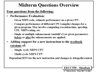
Midterm Questions Overview
- Four questions from the following
- Performance Evaluation
- Given MIPS code, estimate performance on a given
CPU. - Compare performance of different CPU/compiler
changes for a given program. May involve
computing execution time, speedup, CPI, MIPS
rating, etc. - Single or multiple enhancement Amdahls Law given
parameters before or after the enhancements are
applied. - Adding support for a new instruction to the
textbook versions of - Single cycle MIPS CPU
- Multi cycle MIPS CPU
- Dependant RTN for the new instruction and
changes to datapath/control.
2
CPU Organization (Design)
- Datapath Design
- Capabilities performance characteristics of
principal Functional Units (FUs) needed by ISA
instructions - (e.g., Registers, ALU, Shifters, Logic Units,
...) - Ways in which these components are interconnected
(buses connections, multiplexors, etc.). - How information flows between components.
- Control Unit Design
- Logic and means by which such information flow is
controlled. - Control and coordination of FUs operation to
realize the targeted Instruction Set Architecture
to be implemented (can either be implemented
using a finite state machine or a microprogram). - Hardware description with a suitable language,
possibly using Register Transfer Notation (RTN).
Components their connections needed by ISA
instructions
Components
Connections
Control/sequencing of operations of datapath
components to realize ISA instructions
ISA Instruction Set Architecture The ISA forms
an abstraction layer that sets the requirements
for both complier and CPU designers
3
Reduced Instruction Set Computer (RISC)
1984
ISAs
- Focuses on reducing the number and complexity of
instructions of the ISA. - Motivated by simplifying the ISA and its
requirements to - Reduce CPU design complexity
- Improve CPU performance.
- CPU Performance Goal Reduced number of cycles
needed per instruction. At least one
instruction completed per clock cycle. - Simplified addressing modes supported.
- Usually limited to immediate, register indirect,
register displacement, indexed. - Load-Store GPR Only load and store instructions
access memory. - (Thus more instructions are usually executed than
CISC) - Fixed-length instruction encoding.
- (Designed with CPU instruction pipelining in
mind). - Support of delayed branches.
- Examples MIPS, HP PA-RISC, SPARC, Alpha, POWER,
PowerPC.
RISC Goals
(Chapter 2)
4
RISC ISA Example MIPS
R3000 (32-bit)
Registers
- 5 Addressing Modes
- Register direct (arithmetic).
- Immedate (arithmetic).
- Base register immediate offset (loads and
stores). - PC relative (branches).
- Pseudodirect (jumps)
- Operand Sizes
- Memory accesses in any multiple between 1 and 4
bytes.
- Memory Can address 232 bytes
- or 230 words (32-bits).
- Instruction Categories
- Load/Store.
- Computational ALU.
- Jump and Branch.
- Floating Point.
- Using coprocessor
- Memory Management.
- Special.
R0 - R31
31 GPRs R0 0 (each 32 bits)
PC
HI
LO
R-Type
I-Type ALU Load/Store, Branch
J-Type Jumps
Word 4 bytes 32 bits
5
MIPS Register Usage/Naming Conventions
- In addition to the usual naming of registers by
followed with register number, registers are
also named according to MIPS register usage
convention as follows
Register Number Name Usage
Preserved on call?
6
MIPS Five Addressing Modes
- Register Addressing
- Where the operand is a register (R-Type)
- Immediate Addressing
- Where the operand is a constant in the
instruction (I-Type, ALU) - Base or Displacement Addressing
- Where the operand is at the memory location
whose address is the sum of a register and a
constant in the instruction (I-Type, load/store) - PC-Relative Addressing
- Where the address is the sum of the PC and
the 16-address field in the instruction shifted
left 2 bits. (I-Type, branches) - Pseudodirect Addressing
- Where the jump address is the 26-bit jump
target from the instruction shifted left 2 bits
concatenated with the 4 upper bits of the PC
(J-Type)
7
MIPS R-Type (ALU) Instruction Fields
R-Type All ALU instructions that use three
registers
1st operand
2nd operand
Destination
3126 2521 2016
1511 106 50
- op Opcode, basic operation of the instruction.
- For R-Type op 0
- rs The first register source operand.
- rt The second register source operand.
- rd The register destination operand.
- shamt Shift amount used in constant shift
operations. - funct Function, selects the specific variant of
operation in the op field.
Rs, rt , rd are register specifier fields
Independent RTN
Rrd Rrs funct Rrt PC PC 4
Funct field value examples Add 32 Sub 34
AND 36 OR 37 NOR 39
Operand register in rs
Destination register in rd
Operand register in rt
Examples
add 1,2,3 sub 1,2,3
and 1,2,3 or 1,2,3
R-Type Register Type Register Addressing
used (Mode 1)
8
MIPS ALU I-Type Instruction Fields
I-Type ALU instructions that use two registers
and an immediate value (I-Type is also used
for Loads/stores, conditional branches).
1st operand
2nd operand
Destination
3126 2521 2016
150
- op Opcode, operation of the instruction.
- rs The register source operand.
- rt The result destination register.
- immediate Constant second operand for ALU
instruction.
Independent RTN for addi
Rrt Rrs immediate PC PC 4
Source operand register in rs
Result register in rt
OP 8
Constant operand in immediate
OP 12
I-Type Immediate Type Immediate Addressing
used (Mode 2)
9
MIPS Load/Store I-Type Instruction Fields
Base
Src./Dest.
(e.g. offset)
3126 2521 2016
150
Signed address offset in bytes
- op Opcode, operation of the instruction.
- For load word op 35, for store word op 43.
- rs The register containing memory base address.
- rt For loads, the destination register. For
stores, the source register of value to be
stored. - address 16-bit memory address offset in bytes
added to base register.
Examples
MemRrs address Rrt PC PC 4
Store word sw 3, 500(4) Load
word lw 1, 32(2)
Rrt MemRrs address PC PC 4
base register in rs
Destination register in rt
Offset
Base or Displacement Addressing used (Mode 3)
10
MIPS Branch I-Type Instruction Fields
(e.g. offset)
6 bits 5 bits 5 bits
16 bits
3126 2521 2016
150
Signed address offset in words
- op Opcode, operation of the instruction.
- rs The first register being compared
- rt The second register being compared.
- address 16-bit memory address branch target
offset in words added to PC to form branch
address.
Word 4 bytes
Register in rt
offset in bytes equal to instruction address
field x 4
Register in rs
OP 4
Added to PC4 to form branch target
OP 5
Independent RTN for beq
Rrs Rrt PC PC 4 address
x 4 Rrs ¹ Rrt PC PC 4
PC-Relative Addressing used (Mode 4)
11
MIPS J-Type Instruction Fields
J-Type Include jump j, jump and link jal
Jump target in words
3126
250
Word 4 bytes
- op Opcode, operation of the instruction.
- Jump j op 2
- Jump and link jal op 3
- jump target jump memory address in words.
Jump memory address in bytes equal
to instruction field jump target x 4
Effective 32-bit jump address
PC(31-28),jump_target,00
PC(31-28)
From PC4
Independent RTN for j
PC PC 4 PC PC(31-28),jump_target,00
J-Type Jump Type Pseudodirect Addressing used
(Mode 5)
12
MIPS Addressing Modes/Instruction Formats
- All instructions 32 bits wide
Destination
First Operand
Second Operand
Second Operand
First Operand
I-Type
Destination
Base src/dest
Shifted left 2 bits
Pseudodirect Addressing (Mode 5) not shown here,
illustrated in the last slide for J-Type
13
MIPS Arithmetic Instructions Examples
(Integer)
- Instruction Example Meaning Comments
- add add 1,2,3 1 2 3 3 operands
exception possible - subtract sub 1,2,3 1 2 3 3 operands
exception possible - add immediate addi 1,2,100 1 2 100
constant exception possible - add unsigned addu 1,2,3 1 2 3 3
operands no exceptions - subtract unsigned subu 1,2,3 1 2 3 3
operands no exceptions - add imm. unsign. addiu 1,2,100 1 2 100
constant no exceptions - multiply mult 2,3 Hi, Lo 2 x 3 64-bit
signed product - multiply unsigned multu2,3 Hi, Lo 2 x
3 64-bit unsigned product - divide div 2,3 Lo 2 3, Lo quotient, Hi
remainder - Hi 2 mod 3
- divide unsigned divu 2,3 Lo 2
3, Unsigned quotient remainder - Hi 2 mod 3
- Move from Hi mfhi 1 1 Hi Used to get copy of
Hi - Move from Lo mflo 1 1 Lo Used to get copy of
Lo
14
MIPS Logic/Shift Instructions Examples
- Instruction Example Meaning Comment
- and and 1,2,3 1 2 3 3 reg. operands
Logical AND - or or 1,2,3 1 2 3 3 reg. operands
Logical OR - xor xor 1,2,3 1 2 ??3 3 reg. operands
Logical XOR - nor nor 1,2,3 1 (2 3) 3 reg. operands
Logical NOR - and immediate andi 1,2,10 1 2 10 Logical
AND reg, constant - or immediate ori 1,2,10 1 2 10 Logical OR
reg, constant - xor immediate xori 1, 2,10 1 2
10 Logical XOR reg, constant - shift left logical sll 1,2,10 1 2 ltlt
10 Shift left by constant - shift right logical srl 1,2,10 1 2 gtgt
10 Shift right by constant - shift right arithm. sra 1,2,10 1 2 gtgt
10 Shift right (sign extend) - shift left logical sllv 1,2,3 1 2 ltlt 3
Shift left by variable - shift right logical srlv 1,2, 3 1 2 gtgt 3
Shift right by variable - shift right arithm. srav 1,2, 3 1 2 gtgt 3
Shift right arith. by variable
15
MIPS Data Transfer Instructions Examples
- Instruction Comment
- sw 3, 500(4) Store word
- sh 3, 502(2) Store half
- sb 2, 41(3) Store byte
- lw 1, 30(2) Load word
- lh 1, 40(3) Load halfword
- lhu 1, 40(3) Load halfword unsigned
- lb 1, 40(3) Load byte
- lbu 1, 40(3) Load byte unsigned
- lui 1, 40 Load Upper Immediate (16 bits shifted
left by 16)
LUI R5
0000 0000
R5
16
MIPS Branch, Compare, Jump Instructions Examples
- Instruction Example Meaning
- branch on equal beq 1,2,100 if (1 2) go to
PC4100 Equal
test PC relative branch - branch on not eq. bne 1,2,100 if (1! 2) go
to PC4100 Not
equal test PC relative branch - set on less than slt 1,2,3 if (2 lt 3) 11
else 10 -
Compare less than 2s comp. - set less than imm. slti 1,2,100 if (2 lt 100)
11 else 10
Compare lt constant 2s comp. - set less than uns. sltu 1,2,3 if (2 lt 3)
11 else 10 -
Compare less than natural
numbers - set l. t. imm. uns. sltiu 1,2,100 if (2 lt 100)
11 else 10
Compare lt constant natural numbers - jump j 10000 go to 10000
Jump to target address - jump register jr 31 go to 31
For switch, procedure return - jump and link jal 10000 31 PC 4 go to
10000 For
procedure call
17
Example Simple C Loop to MIPS
- Simple loop in C
- Loop g g Ai i i j if (i ! h)
goto Loop - Assume MIPS register mapping
- g s1, h s2, i s3, j
s4, base of A s5 - MIPS Instructions
- Loop add t1,s3,s3 t1 2i add
t1,t1,t1 t1 4i add t1,t1,s5
t1address of AI lw t1,0(t1) t1
Ai add s1,s1,t1 g g Ai add
s3,s3,s4 I i j bne s3,s2,Loop
goto Loop if i!h
A array of words in memory
Word 4 bytes
18
CPU Performance EvaluationCycles Per
Instruction (CPI)
- Most computers run synchronously utilizing a CPU
clock running at a constant clock rate - where Clock rate 1 / clock cycle
- The CPU clock rate depends on the specific CPU
organization (design) and hardware implementation
technology (VLSI) used. - A computer machine (ISA) instruction is comprised
of a number of elementary or micro operations
which vary in number and complexity depending on
the the instruction and the exact CPU
organization (Design). - A micro operation is an elementary hardware
operation that can be performed during one CPU
clock cycle. - This corresponds to one micro-instruction in
microprogrammed CPUs. - Examples register operations shift, load,
clear, increment, ALU operations add , subtract,
etc. - Thus A single machine instruction may take one
or more CPU cycles to complete termed as the
Cycles Per Instruction (CPI). - Average (or effective) CPI of a program The
average CPI of all instructions executed in the
program on a given CPU design.
f 1 / C
Instructions Per Cycle IPC 1/CPI
Cycles/sec Hertz Hz MHz 106 Hz GHz
109 Hz
(Chapter 4)
19
Computer Performance Measures Program
Execution Time
- For a specific program compiled to run on a
specific machine (CPU) A, has the following
parameters - The total executed instruction count of the
program. - The average number of cycles per instruction
(average CPI). - Clock cycle of machine A
- How can one measure the performance of this
machine (CPU) running this program? - Intuitively the machine (or CPU) is said to be
faster or has better performance running this
program if the total execution time is shorter. - Thus the inverse of the total measured program
execution time is a possible performance measure
or metric - PerformanceA 1 /
Execution TimeA - How to compare performance of different machines?
- What factors affect performance? How to improve
performance?
I
CPI
C
Or effective CPI
Seconds/program
Programs/second
20
Comparing Computer Performance Using Execution
Time
- To compare the performance of two machines (or
CPUs) A, B running a given specific program - PerformanceA 1 / Execution TimeA
- PerformanceB 1 / Execution TimeB
- Machine A is n times faster than machine B means
(or slower? if n lt 1) - Example
- For a given program
- Execution time on machine A ExecutionA
1 second - Execution time on machine B ExecutionB
10 seconds - PerformanceA / PerformanceB Execution
TimeB / Execution TimeA -
10 / 1 10 - The performance of machine A is 10 times the
performance of - machine B when running this program, or Machine
A is said to be 10
(i.e Speedup is ratio of performance, no units)
Speedup
The two CPUs may target different ISAs
provided the program is written in a high level
language (HLL)
21
CPU Execution Time The CPU Equation
- A program is comprised of a number of
instructions executed , I - Measured in instructions/program
- The average instruction executed takes a number
of cycles per instruction (CPI) to be completed.
- Measured in cycles/instruction, CPI
- CPU has a fixed clock cycle time C 1/clock
rate - Measured in seconds/cycle
- CPU execution time is the product of the above
three parameters as follows
Or Instructions Per Cycle (IPC)
IPC 1/CPI
C 1 / f
Executed
T I x CPI x
C
execution Time per program in seconds
Number of instructions executed
Average CPI for program
CPU Clock Cycle
(This equation is commonly known as the CPU
performance equation)
22
CPU Execution Time Example
- A Program is running on a specific machine (CPU)
with the following parameters - Total executed instruction count 10,000,000
instructions - Average CPI for the program 2.5
cycles/instruction. - CPU clock rate 200 MHz. (clock cycle C
5x10⁻⁹ seconds) - What is the execution time for this program
- CPU time Instruction count x CPI x Clock
cycle - 10,000,000 x
2.5 x 1 / clock rate - 10,000,000 x
2.5 x 5x10-9 - 0.125 seconds
i.e 5 nanoseconds
T I x CPI x C
Nanosecond nsec ns 10-9 second
23
Factors Affecting CPU Performance
T I
x CPI x C
Instruction Count
Cycles per Instruction
Clock Cycle Time
Program
X
X
X
Compiler
X
Instruction Set Architecture (ISA)
X
X
X
X
Organization (CPU Design)
Technology (VLSI)
X
24
Performance Comparison Example
- From the previous example A Program is running
on a specific machine (CPU) with the following
parameters - Total executed instruction count, I
10,000,000 instructions - Average CPI for the program 2.5
cycles/instruction. - CPU clock rate 200 MHz.
- Using the same program with these changes
- A new compiler used New executed instruction
count, I 9,500,000 - New
CPI 3.0 - Faster CPU implementation New clock rate 300
MHz - What is the speedup with the changes?
- Speedup (10,000,000 x 2.5 x 5x10-9) /
(9,500,000 x 3 x 3.33x10-9 ) - .125 / .095
1.32 - or 32 faster after changes.
Thus C 1/(200x106) 5x10⁻⁹ seconds
Thus C 1/(300x106) 3.33x10⁻⁹ seconds
T I x CPI x C
Clock Cycle C 1/ Clock Rate
25
Instruction Types CPI
- Given a program with n types or classes of
instructions executed on a given CPU with
the following characteristics - Ci Count of instructions of typei
executed - CPIi Cycles per instruction for typei
- Then
- CPI CPU Clock Cycles / Instruction Count
I - Where
- Executed Instruction Count I S Ci
i 1, 2, . n
i.e average or effective CPI
Executed
T I x CPI x C
26
Instruction Types CPI An Example
- An instruction set has three instruction classes
- Two code sequences have the following instruction
counts - CPU cycles for sequence 1 2 x 1 1 x 2 2 x 3
10 cycles - CPI for sequence 1 clock cycles /
instruction count - 10 /5
2 - CPU cycles for sequence 2 4 x 1 1 x 2 1 x 3
9 cycles - CPI for sequence 2 9 / 6 1.5
For a specific CPU design
i.e average or effective CPI
CPI CPU Cycles / I
27
Instruction Frequency CPI
- Given a program with n types or classes of
instructions with the following characteristics - Ci Count of instructions of typei
executed - CPIi Average cycles per instruction of
typei - Fi Frequency or fraction of instruction typei
executed - Ci/ total executed instruction count
Ci/ I - Then
i 1, 2, . n
Where Executed Instruction Count I S Ci
i.e average or effective CPI
Fraction of total execution time for instructions
of type i
T I x CPI x C
28
Instruction Type Frequency CPI A RISC Example
Program Profile or Executed Instructions Mix
Given
Sum 2.2
i.e average or effective CPI
CPI .5 x 1 .2 x 5 .1 x 3 .2 x 2
2.2 .5 1 .3
.4
29
Computer Performance Measures MIPS (Million
Instructions Per Second) Rating
- For a specific program running on a specific CPU
the MIPS rating is a measure of how many millions
of instructions are executed per second - MIPS Rating Instruction count /
(Execution Time x 106) - Instruction count /
(CPU clocks x Cycle time x 106) - (Instruction count
x Clock rate) / (Instruction count x CPI x
106) - Clock rate / (CPI
x 106) - Major problem with MIPS rating As shown above
the MIPS rating does not account for the count of
instructions executed (I). - A higher MIPS rating in many cases may not mean
higher performance or better execution time.
i.e. due to compiler design variations. - In addition the MIPS rating
- Does not account for the instruction set
architecture (ISA) used. - Thus it cannot be used to compare computers/CPUs
with different instruction sets. - Easy to abuse Program used to get the MIPS
rating is often omitted. - Often the Peak MIPS rating is provided for a
given CPU which is obtained using a program
comprised entirely of instructions with the
lowest CPI for the given CPU design which does
not represent real programs.
T I x CPI x C
30
Computer Performance Measures MIPS (Million
Instructions Per Second) Rating
- Under what conditions can the MIPS rating be used
to compare performance of different CPUs? - The MIPS rating is only valid to compare the
performance of different CPUs provided that the
following conditions are satisfied - The same program is used
- (actually this applies to all
performance metrics) - The same ISA is used
- The same compiler is used
- (Thus the resulting programs used to run on the
CPUs and - obtain the MIPS rating are identical at the
machine code level including the same
instruction count)
(binary)
31
Compiler Variations, MIPS Performance An
Example
- For a machine (CPU) with instruction classes
- For a given high-level language program, two
compilers produced the following executed
instruction counts - The machine is assumed to run at a clock rate of
100 MHz.
32
Compiler Variations, MIPS Performance An
Example (Continued)
- MIPS Clock rate / (CPI x 106) 100
MHz / (CPI x 106) - CPI CPU execution cycles / Instructions
count - CPU time Instruction count x CPI / Clock
rate - For compiler 1
- CPI1 (5 x 1 1 x 2 1 x 3) / (5 1 1) 10
/ 7 1.43 - MIPS Rating1 100 / (1.428 x 10⁶) 70.0 MIPS
- CPU time1 ((5 1 1) x 106 x 1.43) / (100 x
106) 0.10 seconds - For compiler 2
- CPI2 (10 x 1 1 x 2 1 x 3) / (10 1 1)
15 / 12 1.25 - MIPS Rating2 100 / (1.25 x 10⁶) 80.0 MIPS
- CPU time2 ((10 1 1) x 106 x 1.25) / (100 x
106) 0.15 seconds
MIPS rating indicates that compiler 2 is
better while in reality the code produced by
compiler 1 is faster
33
MIPS (The ISA not the metric) Loop Performance
Example
- For the loop
- for (i0 ilt1000 ii1)
- xi xi
s - MIPS assembly code is given by
- lw 3, 8(1) load s in 3
- addi 6, 2, 4000 6 address of
last element 4 - loop lw 4, 0(2) load xi in 4
- add 5, 4, 3 5 has xi s
- sw 5, 0(2) store computed
xi - addi 2, 2, 4 increment 2 to
point to next x element - bne 6, 2, loop last loop
iteration reached? - The MIPS code is executed on a specific CPU that
runs at 500 MHz (clock cycle 2ns 2x10⁻⁹
seconds) - with following instruction type CPIs
For this MIPS code running on this CPU find
1- Fraction of total instructions executed for
each instruction type 2- Total number
of CPU cycles 3- Average CPI 4-
Fraction of total execution time for each
instructions type 5- Execution time 6-
MIPS rating , peak MIPS rating for this CPU
Instruction type CPI ALU 4
Load 5 Store 7 Branch 3
X array of words in memory, base address
in 2 , s a constant word value in memory,
address in 1
34
MIPS (The ISA) Loop Performance Example
(continued)
- The code has 2 instructions before the loop and 5
instructions in the body of the loop which
iterates 1000 times, - Thus Total instructions executed, I 5x1000
2 5002 instructions - Number of instructions executed/fraction Fi for
each instruction type - ALU instructions 1 2x1000 2001 CPIALU
4 FractionALU FALU 2001/5002
0.4 40 - Load instructions 1 1x1000 1001 CPILoad
5 FractionLoad FLoad 1001/5002 0.2
20 - Store instructions 1000
CPIStore 7 FractionStore FStore
1000/5002 0.2 20 - Branch instructions 1000
CPIBranch 3 FractionBranch FBranch
1000/5002 0.2 20 - 2001x4
1001x5 1000x7 1000x3 23009 cycles - Average CPI CPU clock cycles / I 23009/5002
4.6 - Fraction of execution time for each instruction
type - Fraction of time for ALU instructions CPIALU x
FALU / CPI 4x0.4/4.6 0.348 34.8 - Fraction of time for load instructions CPIload
x Fload / CPI 5x0.2/4.6 0.217 21.7 - Fraction of time for store instructions
CPIstore x Fstore / CPI 7x0.2/4.6 0.304
30.4 - Fraction of time for branch instructions
CPIbranch x Fbranch / CPI 3x0.2/4.6 0.13
13 - Execution time I x CPI x C CPU cycles x C
23009 x 2x10-9 -
4.6x 10⁻⁵ seconds 0.046 msec 46
usec
Instruction type CPI ALU 4
Load 5 Store 7 Branch 3
35
Performance Enhancement Calculations Amdahl's
Law
- The performance enhancement possible due to a
given design improvement is limited by the amount
that the improved feature is used - Amdahls Law
- Performance improvement or speedup due to
enhancement E - Execution Time
without E Performance with E - Speedup(E) --------------------------------
------ --------------------------------- - Execution Time
with E Performance without E - Suppose that enhancement E accelerates a fraction
F of the execution time by a factor S and the
remainder of the time is unaffected then - Execution Time with E ((1-F) F/S) X
Execution Time without E - Hence speedup is given by
- Execution
Time without E 1 - Speedup(E) -----------------------------------
---------------------- -------------------- - ((1 - F) F/S) X
Execution Time without E (1 - F) F/S
original
F (Fraction of execution time enhanced) refers
to original execution time before the
enhancement is applied
36
Pictorial Depiction of Amdahls Law
Enhancement E accelerates fraction F of original
execution time by a factor of S
Before Execution Time without enhancement E
(Before enhancement is applied)
- shown normalized to 1 (1-F) F 1
After Execution Time with enhancement E
What if the fraction given is after the
enhancement has been applied? How would you solve
the problem? (i.e find expression for speedup)
Execution Time without
enhancement E 1 Speedup(E)
--------------------------------------------------
---- ------------------
Execution Time with enhancement E
(1 - F) F/S
37
Performance Enhancement Example
- For the RISC machine with the following
instruction mix given earlier - Op Freq Cycles CPI(i) Time
- ALU 50 1 .5 23
- Load 20 5 1.0 45
- Store 10 3 .3 14
- Branch 20 2 .4 18
- If a CPU design enhancement improves the CPI of
load instructions from 5 to 2, what is the
resulting performance improvement from this
enhancement - Fraction enhanced F 45 or .45
- Unaffected fraction 100 - 45 55 or .55
- Factor of enhancement 5/2 2.5
- Using Amdahls Law
- 1
1 - Speedup(E) ------------------
--------------------- 1.37 - (1 - F) F/S
.55 .45/2.5
CPI 2.2
38
An Alternative Solution Using CPU Equation
- Op Freq Cycles CPI(i) Time
- ALU 50 1 .5 23
- Load 20 5 1.0 45
- Store 10 3 .3 14
- Branch 20 2 .4 18
- If a CPU design enhancement improves the CPI of
load instructions from 5 to 2, what is the
resulting performance improvement from this
enhancement - Old CPI 2.2
- New CPI .5 x 1 .2 x 2 .1 x 3 .2 x 2
1.6 - Original Execution Time
Instruction count x old CPI x clock
cycle - Speedup(E) -----------------------------------
----------------------------------------
------------------------ - New Execution Time
Instruction count x new CPI x
clock cycle - old CPI 2.2
- ------------ ---------
1.37 -
new CPI
1.6
CPI 2.2
New CPI of load is now 2 instead of 5
T I x CPI x C
39
Performance Enhancement Example
- A program runs in 100 seconds on a machine with
multiply operations responsible for 80 seconds of
this time. By how much must the speed of
multiplication be improved to make the program
four times faster? -
100 - Desired speedup 4
--------------------------------------------------
--- -
Execution Time with enhancement - Execution time with enhancement 100/4
25 seconds
- 25 seconds (100 - 80
seconds) 80 seconds / S - 25 seconds 20 seconds
80 seconds / S - 5 80 seconds / S
- S 80/5 16
- Alternatively, it can also be solved by finding
enhanced fraction of execution time
- F
80/100 .8 - and then solving Amdahls speedup equation for
desired enhancement factor S - Hence multiplication should be 16 times
- faster to get an overall speedup of 4.
1
1
1 Speedup(E) ------------------ 4
----------------- ---------------
(1 - F) F/S (1 -
.8) .8/S .2 .8/s
Solving for S gives S 16
Machine CPU
40
Extending Amdahl's Law To Multiple Enhancements
- Suppose that enhancement Ei accelerates a
fraction Fi of the original execution time by
a factor Si and the remainder of the time is
unaffected then
i 1, 2, . n
Unaffected fraction
What if the fractions given are after the
enhancements were applied? How would you solve
the problem? (i.e find expression for speedup)
Note All fractions Fi refer to original
execution time before the enhancements
are applied.
41
Amdahl's Law With Multiple Enhancements Example
- Three CPU performance enhancements are proposed
with the following speedups and percentage of the
code execution time affected - Speedup1 S1 10 Percentage1
F1 20 - Speedup2 S2 15 Percentage1
F2 15 - Speedup3 S3 30 Percentage1
F3 10 - While all three enhancements are in place in the
new design, each enhancement affects a different
portion of the code and only one enhancement can
be used at a time. - What is the resulting overall speedup?
- Speedup 1 / (1 - .2 - .15 - .1) .2/10
.15/15 .1/30) - 1 / .55
.0333 - 1 / .5833 1.71
42
Pictorial Depiction of Example
Before Execution Time with no enhancements 1
i.e normalized to 1
S1 10
S2 15
S3 30
/ 15
/ 10
/ 30
Unchanged
After Execution Time with enhancements .55
.02 .01 .00333 .5833 Speedup 1 /
.5833 1.71 Note All fractions refer to
original execution time.
What if the fractions given are after the
enhancements were applied? How would you solve
the problem?
43
Reverse Multiple Enhancements Amdahl's Law
- Multiple Enhancements Amdahl's Law assumes that
the fractions given refer to original execution
time. - If for each enhancement Si the fraction Fi it
affects is given as a fraction of the resulting
execution time after the enhancements were
applied then - For the previous example assuming fractions given
refer to resulting execution time after the
enhancements were applied (not the original
execution time), then - Speedup (1 - .2 - .15 - .1) .2
x10 .15 x15 .1x30 - .55
2 2.25 3 - 7.8
Unaffected fraction
i.e as if resulting execution time is normalized
to 1
44
Major CPU Design Steps
- Analyze instruction set to get datapath
requirements - Using independent RTN, write the micro-operations
required for target ISA instructions. - This provides the the required datapath
components and how they are connected. - Select set of datapath components and establish
clocking methodology (defines when storage or
state elements can read and when they can be
written, e.g clock edge-triggered) - Assemble datapath meeting the requirements.
- Identify and define the function of all control
points or signals needed by the datapath. - Analyze implementation of each instruction to
determine setting of control points that affects
its operations. - Control unit design, based on micro-operation
timing and control signals identified - Combinational logic For single cycle CPU.
- Hard-Wired Finite-state machine implementation.
- Microprogrammed.
1
2
Determine number of cycles per instruction and
operations in each cycle.
e.g Any instruction completed in one cycle
45
Datapath Design Steps
- Write the micro-operation sequences required for
a number of representative target ISA
instructions using independent RTN. - Independent RTN statements specify the required
datapath components and how they are connected. - From the above, create an initial datapath by
determining possible destinations for each data
source (i.e registers, ALU). - This establishes connectivity requirements (data
paths, or connections) for datapath components. - Whenever multiple sources are connected to a
single input, a multiplexor of appropriate
size is added. - Find the worst-time propagation delay in the
datapath to determine the datapath clock cycle
(CPU clock cycle). - Complete the micro-operation sequences for all
remaining instructions adding datapath components
connections/multiplexors as needed.
1
2
(or destination)
Or the size of an existing mux is increased
46
Single Cycle MIPS Datapath Extended To Handle
Jump with Control Unit Added
PC 4
PC 4
PC 4
Branch Target
Book figure may have an error!
Opcode
rs
Rrs
rt
Rrt
rd
Rrt
imm16
ALUOp (2-bits) 00 add 01 subtract 10 R-Type
Figure 5.24 page 314
Function Field
This is book version ORI not supported, no zero
extend of immediate needed
47
Control Lines Settings (For Textbook Single
Cycle Datapath including Jump)
Memto- Reg Mem Mem
RegDst ALUSrc Reg
Write Read Write Branch ALUOp1
ALUOp0 Jump R-format 1 0 0 1
0 0 0 1 0 0 lw
0 1 1 1 1 0 0 0
0 0 sw x 1 x 0
0 1 0 0 0 0
beq x 0 x
0 0 0 1 0 1 0 J
x x x 0 0 0 X
x x 1
Similar to Figure 5.18 page 308 with Jump
instruction control line values included
48
Simplified Single Cycle Datapath Timing
- Assuming the following datapath/control hardware
components delays - Memory Units 2 ns
- ALU and adders 2 ns
- Register File 1 ns
- Control Unit lt 1 ns
- Ignoring Mux and clk-to-Q delays, critical path
analysis
Obtained from low-level target VLSI
implementation technology of components
(Load)
Time
0 2ns
3ns 4ns 5ns
7ns
8ns
ns nanosecond 10-9 second
49
Performance of Single-Cycle (CPI1) CPU
- Assuming the following datapath hardware
components delays - Memory Units 2 ns
- ALU and adders 2 ns
- Register File 1 ns
- The delays needed for each instruction type can
be found - The clock cycle is determined by the instruction
with longest delay The load in this case which
is 8 ns. Clock rate 1 / 8 ns 125 MHz - A program with I 1,000,000 instructions
executed takes - Execution Time T I x CPI x C 106
x 1 x 8x10-9 0.008 s 8 msec
Nano second, ns 10-9 second
Load has longest delay of 8 ns thus determining
the clock cycle of the CPU to be 8ns
50
Adding Support for jal to Single Cycle
Datapath(For More Practice Exercise 5.20)
- The MIPS jump and link instruction, jal is used
to support procedure calls by jumping to jump
address (similar to j ) and saving the address
of the following instruction PC4 in register
ra (31) - jal Address
- jal uses the j instruction format
- We wish to add jal to the single cycle datapath
in Figure 5.24 page 314. Add any necessary
datapaths and control signals to the single-clock
datapath and justify the need for the
modifications, if any. - Specify control line values for this instruction.
51
Exercise 5.20 jump and link, jal support to
Single Cycle Datapath
Instruction Word MemPC R31 PC
4 PC Jump Address
Jump Address
PC 4
PC 4
Branch Target
PC 4
rs
Rrs
rt
Rrt
31
2
2
rd
imm16
(For More Practice Exercise 5.20)
52
Adding Control Lines Settings for jal(For
Textbook Single Cycle Datapath including Jump)
Exercise 5.20 jump and link, jal support to
Single Cycle Datapath
MemtoReg Is now 2 bits
RegDst Is now 2 bits
Memto- Reg Mem Mem
RegDst ALUSrc Reg
Write Read Write Branch ALUOp1
ALUOp0 Jump R-format 01 0 00 1
0 0 0 1 0 0 lw
00 1 01 1 1 0 0 0
0 0 sw xx 1 xx 0
0 1 0 0 0 0
beq xx 0 xx
0 0 0 1 0 1 0 J
xx x xx 0 0 0 x
x x 1 JAL 10 x 10
1 0 0 x x x 1
R31
PC 4
PC Jump Address
Instruction Word MemPC R31 PC
4 PC Jump Address
(For More Practice Exercise 5.20)
53
Adding Support for LWR to Single Cycle
Datapath(For More Practice Exercise 5.22)
- We wish to add a variant of lw (load word)
lets call it LWR to the single cycle datapath in
Figure 5.24 page 314. - LWR rd,
rs, rt - The LWR instruction is similar to lw but it sums
two registers (specified by rs, rt) to obtain
the effective load address and uses the R-Type
format - Add any necessary datapaths and control signals
to the single cycle datapath and justify the need
for the modifications, if any. - Specify control line values for this instruction.
Loaded word from memory written to register rd
(For More Practice Exercise 5.22)
54
Adding Control Lines Settings for LWR(For
Textbook Single Cycle Datapath including Jump)
Exercise 5.22 LWR (R-format LW) support to
Single Cycle Datapath
Instruction Word MemPC PC PC
4 Rrd Mem Rrs Rrt
No new components or connections are needed for
the datapath just the proper control line
settings
Memto- Reg Mem Mem
RegDst ALUSrc Reg
Write Read Write Branch ALUOp1
ALUOp0 Jump R-format 1 0 0 1
0 0 0 1 0 0 lw
0 1 1 1 1 0 0 0
0 0 sw x 1 x 0
0 1 0 0 0 0
beq x 0 x
0 0 0 1 0 1 0 J
x x x 0 0 0 x
x x 1 LWR 1 0 1
1 1 0 0 0 0 0
Add
Rrt
rd
(For More Practice Exercise 5.22)
55
Adding Support for jm to Single Cycle
Datapath(Based on For More Practice Exercise
5.44 but for single cycle)
- We wish to add a new instruction jm (jump
memory) to the single cycle datapath in Figure
5.24 page 314. - jm
offset(rs) - The jm instruction loads a word from effective
address (Rrs offset), this is similar to lw
except the loaded word is put in the PC instead
of register rt. - Jm used the I-format with field rt not used.
- Add any necessary datapaths and control signals
to the single cycle datapath and justify the need
for the modifications, if any. - Specify control line values for this instruction.
56
Adding jump memory, jm support to Single Cycle
Datapath
Instruction Word MemPC PC MemRrs
SignExtimm16
Jump
2
2
PC 4
Jump
2
Branch Target
rs
Rrs
rt
Rrt
rd
imm16
(Based on For More Practice Exercise 5.44 but
for single cycle)
57
Adding Control Lines Settings for jm(For
Textbook Single Cycle Datapath including Jump)
Adding jm support to Single Cycle Datapath
Jump is now 2 bits
Memto- Reg Mem Mem
RegDst ALUSrc Reg
Write Read Write Branch ALUOp1
ALUOp0 Jump R-format 1 0 0 1
0 0 0 1 0 00 lw
0 1 1 1 1 0 0
0 0 00 sw x 1 x
0 0 1 0 0 0 00
beq x 0
x 0 0 0 1 0 1 00
J x x x 0 0 0
x x x 01 Jm x 1
x 0 1 0 x 0 0
10
add
PC MemRrs SignExtimm16
58
Reducing Cycle Time Multi-Cycle Design
- Cut combinational dependency graph by inserting
registers / latches. - The same work is done in two or more shorter
cycles, rather than one long cycle.
storage element
storage element
Two shorter cycles
Acyclic Combinational Logic (A)
One long cycle
Cycle 1
Acyclic Combinational Logic
e.g CPI 1
e.g CPI 2
gt
storage element
Acyclic Combinational Logic (B)
Cycle 2
storage element
- Place registers to
- Get a balanced clock cycle length
- Save any results needed for the remaining cycles
storage element
59
Alternative Multiple Cycle Datapath With Control
Lines (Fig 5.28 In Textbook)
(Figure 5.28 page 323)
60
Operations (Dependant RTN) for Each Cycle
Load IR MemPC PC PC 4
A Rrs B Rrt ALUout PC
(SignExt(imm16) x4) ALUout A
SignEx(Imm16) MDR MemALUout
Rrt MDR
Store IR MemPC PC PC 4
A Rrs B Rrt ALUout PC
(SignExt(imm16) x4) ALUout
A SignEx(Imm16) MemALUout
B
Jump IR MemPC PC PC 4 A
Rrs B Rrt ALUout PC
(SignExt(imm16) x4) PC Jump Address
R-Type IR MemPC PC PC 4 A
Rrs B Rrt ALUout PC
(SignExt(imm16) x4) ALUout A
funct B Rrd ALUout
Branch IR MemPC PC PC 4
A Rrs B Rrt ALUout PC
(SignExt(imm16) x4) Zero A - B Zero PC
ALUout
Instruction Fetch
IF ID EX MEM WB
Instruction Decode
Execution
Memory
Write Back
Instruction Fetch (IF) Instruction Decode (ID)
cycles are common for all instructions
61
Multi-cycle Datapath Instruction CPI
- R-Type/Immediate Require four cycles, CPI 4
- IF, ID, EX, WB
- Loads Require five cycles, CPI 5
- IF, ID, EX, MEM, WB
- Stores Require four cycles, CPI 4
- IF, ID, EX, MEM
- Branches/Jumps Require three cycles, CPI 3
- IF, ID, EX
- Average or effective program CPI 3 CPI
5 depending on program profile
(instruction mix).
62
FSM State Transition Diagram (From Book)
IF
A Rrs B Rrt ALUout PC
(SignExt(imm16) x4)
ID
(Figure 5.37 page 338)
IR MemPC PC PC 4
ALUout A SignEx(Imm16)
PC Jump Address
EX
ALUout A func B
Zero A -B Zero PC ALUout
MDR MemALUout
WB
MEM
Rrd ALUout
MemALUout B
Total 10 states
Rrt MDR
WB
63
MIPS Multi-cycle Datapath Performance Evaluation
- What is the average CPI?
- State diagram gives CPI for each instruction type
- Workload below gives frequency of each type
Type CPIi for type Frequency CPIi x freqIi
Arith/Logic 4 40 1.6 Load 5
30 1.5 Store 4 10 0.4 branch
3 20 0.6 Average
CPI 4.1
Better than CPI 5 if all instructions took the
same number of clock cycles (5).
T I x CPI x C
64
Adding Support for swap to Multi Cycle Datapath
(For More Practice Exercise 5.42)
- You are to add support for a new instruction,
swap that exchanges the values of two registers
to the MIPS multicycle datapath of Figure 5.28 on
page 232 - swap rs, rt
- Swap used the R-Type format with
- the value of field rs the
value of field rd - Add any necessary datapaths and control signals
to the multicycle datapath. Find a solution that
minimizes the number of clock cycles required for
the new instruction without modifying the
register file. Justify the need for the
modifications, if any. - Show the necessary modifications to the
multicycle control finite state machine of Figure
5.37 on page 338 when adding the swap
instruction. For each new state added, provide
the dependent RTN and active control signal
values.
i.e No additional register write ports
65
Adding swap Instruction Support to Multi Cycle
Datapath
We assume here rs rd in instruction encoding
Swap rs, rt Rrt Rrs
Rrs
Rrt
PC 4
rs
Branch Target
Rrs
rt
Rrt
rd
imm16
The outputs of A and B should be connected to the
multiplexor controlled by MemtoReg if one of the
two fields (rs and rd) contains the name of one
of the registers being swapped. The other
register is specified by rt. The MemtoReg
control signal becomes two bits.
(For More Practice Exercise 5.42)
66
Adding swap Instruction Support to Multi Cycle
Datapath
IF
A Rrs B Rrt ALUout PC
(SignExt(imm16) x4)
ID
IR MemPC PC PC 4
EX
ALUout A SignEx(Im16)
WB1
Rrd B
ALUout A func B
WB2
Zero A -B Zero PC ALUout
Rrt A
Rrd ALUout
MEM
WB
MDR MemALUout
MemALUout B
Swap takes 4 cycles
Rrt MDR
WB
67
Adding Support for add3 to Multi Cycle
Datapath(For More Practice Exercise 5.45)
- You are to add support for a new instruction,
add3, that adds the values of three registers,
to the MIPS multicycle datapath of Figure 5.28 on
page 232 For example - add3 s0,s1, s2, s3
- Register s0 gets the sum of s1, s2
and s3. - The instruction encoding uses a modified
R-format, with an additional register specifier
rx added replacing the five low bits of the
funct field. - Add necessary datapath components, connections,
and control signals to the multicycle datapath
without modifying the register bank or adding
additional ALUs. Find a solution that minimizes
the number of clock cycles required for the new
instruction. Justify the need for the
modifications, if any. - Show the necessary modifications to the
multicycle control finite state machine of Figure
5.37 on page 338 when adding the add3
instruction. For each new state added, provide
the dependent RTN and active control signal
values.
68
Exercise 5.45 add3 instruction support to
Multi Cycle Datapath
Add3 rd, rs, rt, rx Rrd
Rrs Rrt Rrx
rx is a new register specifier in field 0-4 of
the instruction No additional register read ports
or ALUs allowed
Modified R-Format
WriteB
2
PC 4
rs
Branch Target
rt
rx
rd
imm16
1. ALUout is added as an extra input to first ALU
operand MUX to use the previous ALU result as an
input for the second addition. 2. A multiplexor
should be added to select between rt and the new
field rx containing register number of the 3rd
operand (bits 4-0 for the instruction) for input
for Read Register 2. This multiplexor will be
controlled by a new one bit control signal called
ReadSrc.
3. WriteB control line added to enable writing
Rrx to B
69
Exercise 5.45 add3 instruction support to
Multi Cycle Datapath
IF
A Rrs B Rrt ALUout PC
(SignExt(imm16) x4)
ID
IR MemPC PC PC 4
EX
WriteB
ALUout A SignEx(Im16)
EX1
ALUout A B B Rrx
WriteB
ALUout A func B
EX2
Zero A -B Zero PC ALUout
MDR MemALUout
ALUout ALUout B
Rrd ALUout
MEM
WB
MemALUout B
Add3 takes 5 cycles
Rrt MDR
WB
(For More Practice Exercise 5.45)
Recommended
CrystalGraphics Presentations


