OCCULAR

1
OCCULAR

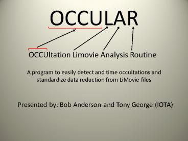
• OCCUltation Limovie Analysis Routine

A program to easily detect and time occultations
and standardize data reduction from LiMovie files
Presented by Bob Anderson and Tony George (IOTA)
2
Motivation for OCCULAR how to deal with noise

• Above is a plot from a LiMovie processed
  occultation event. One would like to
• Locate a likely occultation event that is
  obscured by noise
• Calculate D and R in a standardized manner
• Use statistics to gain confidence that the
  event is not noise

3
The good news is that the troublesome noise is
gaussian (normal distribution)

• Because the noise is gaussian, we are on solid
  ground to use
• Standard least-squares estimates of event
  parameters
• Standard statistical confidence measures

4
Another piece of good news.In the absence of
noise, we expect our observations to look like
one of the idealized data traces shown below
and since we know the expected shape of our
event, we can use standard techniques from
signal processing theory to locate where in the
data our event is positioned.
5
Occular nomenclature and conventions
event
wing
wing
b
a
transition
wing 17 readings event 4
readings transition 2 readings
is how the above shape would be specified
This alternative way of setting shape width is
also available
event (FWHM) 7 readings
The values for b (baseline) and a (asteroid) are
output values determined by least-squares fit
Note D, R, and duration are reported at FWHM
If that is not appropriate, the user will have to
manually calculate these numbers from the
available data.
6
The OCCULAR algorithm pseudo-code

• Accept user input to define a range of ideal
  signal shapes (min max for event width and
  transition, and wing size)
• for each (signal)
• position signal at the left edge of the
  input data
• set max FOM found to zero
• do
• calculate a figure of merit (FOM) for
  how well signal matches data
• calculate least-squares value for the
  event parameters
• calculate statistical measures of the
  fit (Tstat)
• keep track of the max FOM found so far
  (and associated information)
• slide the signal one step to the right
• until (signal is at right edge of input
  data)
• add the data found at max FOM to the maxFOM
  list
• Look through the maxFOM list and highlight the
  list entry that contains the max maxFOM value.
  This is the found event.
• Display a plot of the results.

7
FOM (figure of merit) calculation
This is a standard technique used to locate the
position of a known signal (x) in a noisy data
stream (y) Note the datai and signali have
been adjusted to have a mean of zero before the
following code is executed. leftIndex and
rightIndex deal with the occasions where some
part of the signal lies outside the input data.

• // Calculate the normalized correlation
  coefficient.
• double xySum 0.0
• double yySum 0.0
• double xxSum 0.0
• for (i leftIndex i lt
  rightIndex i)
• xySum datai
  signali
• yySum datai
  datai
• xxSum signali
  signali
• fom xySum / (Sqrt(xxSum)
  Sqrt(yySum))
• if (fom lt 0) fom 0.0

8
Our main statistical measure (Students t)
n1 number of readings in wings n2 number of
readings at the bottom of the event S2x
variance of X (the b value of our signal) S2y
variance of Y (the a value of our signal) df
degrees of freedom Note we do NOT include
readings in the transition zone in the
calculation of T
9
A visual to give substance to the earlier
discussion
10
Tstat
Position of event
Width of event (1 to 250)
Cancri Tstat surface (perspective view)
11
Width of event (1 to 250)
Position of event
A view of Cancri Tstat surface from above
12

• In a moment, Tony George is going to demonstrate
  OCCULAR.
• He will begin by showing the program at work on
  the Hiraoka data.
• Unlike the Cancri event, which was clearly
  detected, the Hiraoka data is an example where
  one must spend more time answering the question
• Did we really observe an occultation event,
  or was that just noise?
• The following two slides illustrate the issue.

13
FOM
Position of event
Width of event
Hiraoka FOM surface
This shows an event that is similar to noise
FOM may be somewhat ambiguous, but Tstat tells a
different story
14
This event is now more clearly distinguished
Tstat
Position of event
Width of event (1 to 100)
Hiraoka Tstat surface
15

• And now Tony will demonstrate the program in
  action on real data.