Polynomial Approximation

1
Polynomial Approximation

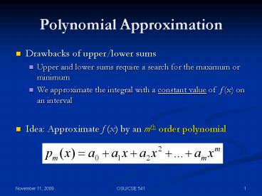
• Drawbacks of upper/lower sums
• Upper and lower sums require a search for the
  maximum or minimum
• We approximate the integral with a constant value
  of f (x) on an interval
• Idea Approximate f (x) by an mth order
  polynomial

2
Newton-Cotes Formulas

• Different choices for ms lead to different
  formulas
• The ms (order of the polynomials) may be the
  same or different over each interval
• Lets assume it is the same over all intervals
  for now

3
Trapezoid Rule

• Simplest way to approximate the area under a
  curve using first order polynomial (a straight
  line)
• Using Newtons form of the interpolating
  polynomial
• Now, solve for the integral

4
Trapezoid Rule
Trapezoid Rule
5
Trapezoid Rule

• Is this really an improvement?

6
Trapezoid Rule Error

• The integration error is (assume equal spaced
  subdivision)
• where, h (b a)/n and ? is an unknown point (
  a lt ? lt b ) (Intermediate Value Theorem)
• What if the function, f, is linear
• Exact integration why?
• f?? 0

7
More intervals, better result error ? O(h2)
8
Composite Trapezoid Rule

• Consider the interval a, b
• Break up the interval into n 1 equally spaced
  points.
• Let
• Each interval has

9
Composite Trapezoid Rule

• Substitute the trapezoid rule for each integral
• Results in the Composite Trapezoid Formula

10
Composite Trapezoid Rule

• Note Multiple intervals allow us to avoid
  duplicate function evaluations and operations
• The width times the average height

11
Error Analysis

• The error can be estimated as
• Where, is the average second derivative.
• If n is doubled
• h ? h/2 and Ea ? Ea/4
• The error depends on the width of the area of
  integration

12
Example

• Integrate
• a, b 0.2, 0.8

Analytical Answer 12.82
13
Example

• Apply the Trapezoid Rule once
• Error

14
Example

• We dont know ? so approximate with avg. f??

15
Example

• The error can thus be estimated as

16
Trapezoid rule approximation of 11.26 with error
2.37 is within 12 of the true answer
17
Three Intervals

• Use intervals (0.2, 0.4),(0.4, 0.6),(0.6, 0.8)
• (n 3, h 0.2)

Analytical answer is 12.82
18
Et is now within 2
19
Six Intervals

• Use intervals (0.2, 0.3),(0.3, 0,4), etc.
• (n 6, h 0.1)

Analytical answer is 12.82
20
Et is now 0.5
21
Can We Do Better?

• Recap
• Riemann sum
• Trapezoid rule
• What ways can we improve our estimate? Ideas?
• More intervals
• Higher order polynomial
• Use Richardson Extrapolation to examine the limit
  as h ? 0

22
Adding More Intervals

• Take the Composite Trapezoid Rule
• Assume we have computed an estimate with interval
  size h
• Observation Why dont we need to recompute
  everything for interval size h/2?

23
Recursive Trapezoid Rule

• We have n? 2n and h?h/2

We computed this already!
24
Romberg Integration

• This is called Romberg Integration
• We combined two O(h2) estimates to get an O(h4)
  estimate
• Continue by combining two O(h4) estimates to get
  an O(h6) estimate
• Continue by combining two O(h6) estimates to get
  an O(h8) estimate

25
Romberg Integration

• Greater weight is placed on the more accurate
  estimate
• Weighting coefficients sum to unity
• i.e, (16-1)/151

26
Romberg Integration

• Recursive definition
• j level of subdivision, j1 has more intervals
• k level of integration
• k 1 is original trapezoid estimate O(h2)
• k 2 is improved O(h4), etc.

27
Example

• Consider the function
• Integrate from a 0 to b 0.8

28
Example

• Trapezoid Rules

k 0
k 1
k
j
j 0
j 1
j 2
(j1, k1)
Exact integral is 1.64053334
29
Example
k 1
k 0
k
j
(j2, k1)
Exact integral is 1.64053334
30
Example
k 2
k 1
k
j
(j2, k2)
Exact integral is 1.64053334
31
Example
k
k 1
k 3
k 2
j
Exact integral is 1.64053334
32
Example

• Continue for better results

k 3
(j3, k3)
33
Multi-dimensional Integration

• Apply the Trapezoid Rule to a two-dimensional
  function
• This leads to weights in the following pattern

34
Multi-dimensional Integration

• Let Aij be the weights to the function evals

35
Multi-dimensional Integration

• The integration in 2D with the Composite
  Trapezoid rule

36
Multi-dimensional Integration

• Observations
• Using the weights from the Trapezoid rule still
  leaves the error as O(h2)
• However, there are now n2 function evaluations
• Equally-spaced samples on a square region

37
Multi-dimensional Integration

• In general, given k dimensions, we have N nk
  function evaluations
• If the dimension is high, this leads to a
  significant amount of additional work in going
  from h?h/2.
• Note remember this for Monte-Carlo Integration.