
Stochastic%20Network%20Optimization - PowerPoint PPT Presentation
Title:
Stochastic%20Network%20Optimization
Description:
Stochastic Network Optimization (a 1-day short course) Michael J. Neely ... Lee, Mazumdar, Shroff [2005] (Stochastic Gradients) Lin, Shroff [2004] (Scheduling ... – PowerPoint PPT presentation
Number of Views:132
Avg rating:3.0/5.0
Title: Stochastic%20Network%20Optimization
1
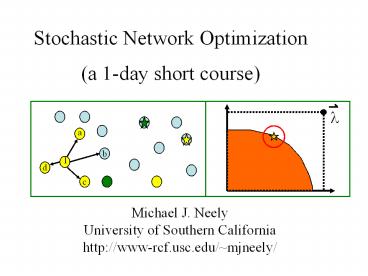
Stochastic Network Optimization (a 1-day short
course)
l
a
b
1
d
c
Michael J. Neely University of Southern
California http//www-rcf.usc.edu/mjneely/
2
Lectures based on the following text L.
Georgiadis, M. J. Neely, L. Tassiulas, Resource
Allocation And Cross-Layer Control in Wireless
Networks, Foundations And Trends in Networking,
vol. 1, no. 1, pp. 1-144, 2006. Free PDF
download of text on the following web pages
http//www-rcf.usc.edu/mjneely/ A hardcopy
can be ordered for around 50 from NOW
publishers
3
A brief history of Lyapunov Drift for Queueing
Systems
Lyapunov Stability Tassiulas, Ephremides 91,
92, 93 P. R. Kumar, S. Meyn 95 McKeown,
Anantharam, Walrand 96, 99 Kahale, P. E. Wright
97 Andrews, Kumaran, Ramanan, Stolyar, Whiting
2001 Leonardi, Mellia, Neri, Marsan
2001 Neely, Modiano, Rohrs 2002, 2003, 2005
Joint Stability with Utility Optimization was the
Big Open Question until Tsibonis,
Georgiadis, Tassiulas infocom 2003 (special
structure net,
linear utils) Neely, Modiano thesis 2003,
infocom 2005 (general nets and utils)
Eryilmaz, Srikant infocom 2005 (downlink,
general utils) Stolyar Queueing Systems 2005
(general nets and utils)
4
Lyapunov drift for joint stability and
performance optimization Neely, Modiano 2003,
2005 (Fairness, Energy) Georgiadis, Neely,
Tassiulas NOW Publishers, FT, 2006 Neely
Infocom 2006, JSAC 2006 (Super-fast delay
tradeoffs) Alternate Approaches to Stoch.
Performance Optimization Tsibonis, Georgiadis,
Tassiulas 2003 (special structure net,
linear utils) Eryilmaz, Srikant 2005
(Fluid Model Transformations) Stolyar 2005
(Fluid Model Transformations) Lee, Mazumdar,
Shroff 2005 (Stochastic Gradients) Lin, Shroff
2004 (Scheduling for static channels)
5
Lyapunov drift for joint stability and
performance optimization Neely, Modiano 2003,
2005 (Fairness, Energy) Georgiadis, Neely,
Tassiulas NOW Publishers, FT, 2006 Neely
Infocom 2006, JSAC 2006 (Super-fast delay
tradeoffs) Alternate Approaches to Stoch.
Performance Optimization Tsibonis, Georgiadis,
Tassiulas 2003 (special structure net,
linear utils) Eryilmaz, Srikant 2005
(Fluid Model Transformations) Stolyar 2005
(Fluid Model Transformations) Lee, Mazumdar,
Shroff 2005 (Stochastic Gradients) Lin, Shroff
2004 (Scheduling for static channels)
Yields Explicit Delay Tradeoff Results!
6
lij
Network Model --- The General Picture
Flow Control Decision Rij(t)
own
other
- 3 Layers
- Flow Control (Transport)
- Routing (Network)
- Resource Alloc./Sched. (MAC/PHY)
From Resource Allocation and Cross-Layer
Control in Wireless Networks by Georgiadis,
Neely, Tassiulas, NOW Foundations and Trends in
Networking, 2006
7
Network Model --- The General Picture
own
other
- 3 Layers
- Flow Control (Transport)
- Routing (Network)
- Resource Alloc./Sched. (MAC/PHY)
From Resource Allocation and Cross-Layer
Control in Wireless Networks by Georgiadis,
Neely, Tassiulas, NOW Foundations and Trends in
Networking, 2006
8
Network Model --- The General Picture
own
other
Data Pumping Capabilities (mij(t)) C(I(t),
S(t))
Control Action (Resource Allocation/Power)
Channel State Matrix
- 3 Layers
- Flow Control (Transport)
- Routing (Network)
- Resource Alloc./Sched. (MAC/PHY)
I(t) I
From Resource Allocation and Cross-Layer
Control in Wireless Networks by Georgiadis,
Neely, Tassiulas, NOW Foundations and Trends in
Networking, 2006
9
DIVBAR for Mobile Networks
10
DIVBAR for Mobile Networks
11
DIVBAR for Mobile Networks
12
DIVBAR for Mobile Networks
13
DIVBAR for Mobile Networks
14
DIVBAR for Mobile Networks
15
DIVBAR for Mobile Networks
16
DIVBAR for Mobile Networks
17
DIVBAR for Mobile Networks
18
DIVBAR for Mobile Networks
19
DIVBAR for Mobile Networks
20
Application 3 Mesh Networks
Communiation Pairs 0 1, 2 3, ,
8 9
Halfway through the simulation, node 0 moves
(non-ergodically) from its initial location to
its final location. Node 9 takes a Markov Random
walk.
0
1
2
8
4
7
6
3
5
9
Full throughput is maintained throughout, with
noticeable delay increase (at new equilibrium),
but which is independent of mobility timescales.
21
More simulation results for the mesh
network Flow control included (determined by
parameter V)
22
- Course Outline
- Intro and Motivation (done)
- Magic of Telescoping Sums
- Discrete Time Queues
- 4. Stability and Capacity Regions
- 5. Lyapunov Drift
- Max-Weight Algorithms for Stability
- (imperfect scheduling, robust to
non-ergodic traffic) - (downlinks, backpressure, multi-hop,
mobile) - Lyapunov Drift with Performance Optimization
- 8. Energy Problems
- Virtual Queues and Power Constraints
- General Constrained Optimization
- 11. Other Utilities Flow control and Fairness
- 12. Modern Network Models
23
A (very un-impressive) Magic Trick
5
12
1
11
-3
8
9
?
7
24
A (very un-impressive) Magic Trick
5
12 - 5 7
12
1
11
-3
8
9
?
7
25
A (very un-impressive) Magic Trick
5
12 - 5 7 11 - 12 -1
12
1
11
-3
8
9
?
7
26
A (very un-impressive) Magic Trick
5
12 - 5 7 11 - 12 -1 8 - 11 -3
12
1
11
-3
8
9
?
7
27
A (very un-impressive) Magic Trick
5
- 12 - 5 7
- 11 - 12 -1
- - 11 -3
- ? - 8 ??
12
1
11
-3
8
9
?
7
28
A (very un-impressive) Magic Trick
5
- 12 - 5 7
- 11 - 12 -1
- - 11 -3
- ? - 8 ??
- 7 - ? ??
12
1
11
-3
8
9
?
7
29
A (very un-impressive) Magic Trick
5
- 12 - 5 7
- 11 - 12 -1
- - 11 -3
- ? - 8 ??
- - ? ??
- 9 - 7 2
12
1
11
-3
8
9
?
7
30
A (very un-impressive) Magic Trick
5
- 12 - 5 7
- 11 - 12 -1
- - 11 -3
- ? - 8 ??
- - ? ??
- - 7 2
- -3 - 9 -12
12
1
11
-3
8
9
?
7
31
A (very un-impressive) Magic Trick
5
- 12 - 5 7
- 11 - 12 -1
- - 11 -3
- ? - 8 ??
- - ? ??
- - 7 2
- -3 - 9 -12
- 1 - (-3) 4
12
1
11
-3
8
9
?
7
32
A (very un-impressive) Magic Trick
5
- 12 - 5 7
- 11 - 12 -1
- - 11 -3
- ? - 8 ??
- - ? ??
- - 7 2
- -3 - 9 -12
- 1 - (-3) 4
- 5 - 1 4
12
1
11
-3
8
9
?
7
33
A (very un-impressive) Magic Trick
5
- 12 - 5 7
- 11 - 12 -1
- - 11 -3
- ? - 8 ??
- - ? ??
- - 7 2
- -3 - 9 -12
- 1 - (-3) 4
- 5 - 1 4
12
1
11
-3
8
9
?
7
34
A (very un-impressive) Magic Trick
5
- 12 - 5 7
- 11 - 12 -1
- - 11 -3
- 2 - 8 -6
- - 2 5
- - 7 2
- -3 - 9 -12
- 1 - (-3) 4
- 5 - 1 4
- 0
12
1
11
-3
Zero!
8
9
?2
7
35
A (very un-impressive) Magic Trick
5
- 12 - 5 7
- 11 - 12 -1
- - 11 -3
- 2 - 8 -6
- - 2 5
- - 7 2
- -3 - 9 -12
- 1 - (-3) 4
- 5 - 1 4
- 0
12
1
11
-3
Zero!
8
9
?2
7
36
A (very un-impressive) Magic Trick
5
- 12 - 5 7
- 11 - 12 -1
- - 11 -3
- 2 - 8 -6
- - 2 5
- - 7 2
- -3 - 9 -12
- 1 - (-3) 4
- 5 - 1 4
- 0
12
1
11
-3
Zero!
8
9
?2
7
37
A (very un-impressive) Magic Trick
5
- 12 - 5 7
- 11 - 12 -1
- - 11 -3
- 2 - 8 -6
- - 2 5
- - 7 2
- -3 - 9 -12
- 1 - (-3) 4
- 5 - 1 4
- 0
12
1
11
-3
Zero!
8
9
?2
7
38
A (very un-impressive) Magic Trick
5
- 12 - 5 7
- 11 - 12 -1
- - 11 -3
- 2 - 8 -6
- - 2 5
- - 7 2
- -3 - 9 -12
- 1 - (-3) 4
- 5 - 1 4
- 0
12
1
11
-3
Zero!
8
9
?2
7
39
Fact (Telescoping Sums) Let t 0, 1, 2, 3,
Let f(t) be any function of discrete time
t Define D(t) f(t1) - f(t)
(difference) Then D(t) f(M)
- f(0)
M-1
t0
f(1)-f(0) f(2)-f(1) f(3)-f(2)
D(M-1)
D(0)
D(1)
D(2)
D(M-2)
0
1
2
3
M-2
M-1
M
40
A single discrete time queue
U(t)
m(t)
A(t)
Discrete time t 0, 1, 2, U(t) Queue
Backlog (Unfinished Work) at
time t units bits, real number A(t)
Arrivals during slot t m(t) Transmission
rate on slot t (bits/slot)
41
A single discrete time queue
U(t)
m(t)
A(t)
Discrete time t 0, 1, 2, U(t) Queue
Backlog (Unfinished Work) at
time t units bits, real number A(t)
Arrivals during slot t m(t) Transmission
rate on slot t (bits/slot)
Alternate Units U(t) packets (integer), m(t)
packets/slot
42
A single discrete time queue
U(t)
m(t)
A(t)
Dynamic Equation
U(t1) maxU(t) - m(t), 0 A(t)
43
A single discrete time queue
U(t)
m(t)
A(t)
Dynamic Equation
U(t1) maxU(t) - m(t), 0 A(t)
ltORgt
U(t1) U(t) - m(t) A(t)
44
A single discrete time queue
U(t)
m(t)
A(t)
Dynamic Equation
U(t1) maxU(t) - m(t), 0 A(t)
ltORgt
U(t1) U(t) - m(t) A(t)
(where m(t) ?? )
45
A single discrete time queue
U(t)
m(t)
A(t)
Dynamic Equation
U(t1) maxU(t) - m(t), 0 A(t)
ltORgt
U(t1) U(t) - m(t) A(t)
(where m(t) minm(t) , U(t) )
46
U(t)
m(t)
A(t)
U(t1) U(t) - m(t) A(t) U(t1) - U(t) A(t)
- m(t)
()
gt
Basic Sample Path Equality (t1 lt t2)
U(t2) - U(t1) A(t) - m(t)
Proof Use equation () with the telescoping
sums fact.
47
A(t)
m(t)
U(t)
Important Sample Path Equality and Inequalities
U(t2) - U(t1) A(t) - m(t)
U(t2) - U(t1) A(t) - m(t)
gt
U(t) A(t) - m(t)
gt
(if U(0) 0)
48
A(t)
m(t)
U(t)
A(t), m(t) are Discrete time Stochastic Processes
(t 0, 1, 2, )
Queue Stability A discrete time queue U(t) is
strongly stable if
1
lim sup
EU(t)
lt
t
49
A(t)
m(t)
U(t)
A(t), m(t) are Discrete time Stochastic Processes
(t 0, 1, 2, )
call this stability for simplicity
Queue Stability A discrete time queue U(t) is
strongly stable if
1
lim sup
EU(t)
lt
t
Define this as U
50
Theorem If m(t) lt mmax for all t, and if U(t)
is strongly stable, then
EU(t)
0
t
Proof See Appendix D of M. J. Neely, Energy
Optimal Control for Time Varying Wireless
Networks, IEEE Transactions on Information
Theory, vol. 52, no. 7, July 2006.
51
Corollary Suppose m(t) lt mmax for all t, and
(1)
(2)
Then if U(t) is strongly stable, we must have
Necessary Condition for Stability (intuitive)
mav
l
52
Proof We know that (assuming U(0)0)
U(t) A(t) - m(t)
-Take Expectations
53
Proof We know that (assuming U(0)0)
EU(t) EA(t) - Em(t)
-Take Expectations -Divide by t
54
Proof We know that (assuming U(0)0)
EA(t) -
Em(t)
-Take Expectations -Divide by t -Take limits
55
Proof We know that (assuming U(0)0)
EA(t) -
Em(t)
0 l - mav
-Take Expectations -Divide by t -Take limits
56
Corollary (Alternate form) Suppose m(t) lt
mmax for all t. Then if U(t) is strongly
stable, we must have
1
lim inf
Em(t) - A(t) 0
t
Holds in cases when time averages of A(t) and/or
m(t) do not necessarily exist. Proof similar
(exercise).
57
Thus (assuming l, mav are defined)
is a necessary condition for stability.
We want a sufficient condition for
stability (need more structure on A(t), m(t))
58
Arrival Process A(t) is admissible with rate l
if
2
EA(t)2 H(t) Amax
(some Amax lt )
For any dgt0, there is a T such that for any t0
t
H(t) Past History up to time t
59
Server Process m(t) is admissible with rate m
if
(some mmax lt )
m(t) mmax for all t
For any dgt0, there is a T such that for any t0
E m - d
t
H(t) Past History up to time t
60
Fact iid probabilistic splitting (with
probability p) of an admissible process A(t)
with rate l yields an admissible process of rate
pl.
Asplit(t) pl
A(t) l
p
1-p
Asplit(t) A(t) with prob p, 0 else.
Proof Simple Exercise
61
Theorem (Queue Stability) Suppose that
A(t) is admissible with rate l
m(t) is admissible with rate m
Then
(a) l m is necessary for stability of
U(t)
(b) l lt m is sufficient for stability of
U(t)
62
Theorem (Queue Stability) Suppose that
A(t) is admissible with rate l
m(t) is admissible with rate m
Then
(a) l m is necessary for stability of
U(t)
(b) l lt m is sufficient for stability of
U(t)
Proof of (b) T-slot Lyapunov drift, Lemma 4.4
of text
63
Definition A network of queues is strongly
stable if all individual queues are strongly
stable.
64
A simple routing problem for two queues
m1
U1(t)
A(t)
(admissible, rate l)
m2
U2(t)
Rules (1) Every slot t, must put all new A(t)
arrivals of that slot to either queue 1 or
queue 2. (2) Must make decision immediately (no
data storage at the decision point).
65
A simple routing problem for two queues
m1
U1(t)
A(t)
(admissible, rate l)
m2
U2(t)
Definition The Capacity Region L is the
closure of the set of all rates l for which a
stabilizing routing algorithm exists (subject to
the given rules).
66
A simple routing problem for two queues
m1
U1(t)
A(t)
(admissible, rate l)
m2
U2(t)
Claim L l 0 l m1 m2
l
m1 m2
0
67
A simple routing problem for two queues
m1
U1(t)
A(t)
(admissible, rate l)
m2
U2(t)
Claim L l 0 l m1 m2
Must show 2 things
l lt m1 m1 sufficient
(i)
(ii)
l
m1 m2
0
68
A(t)
(admissible, rate l)
Proof of Necessity Under any routing
algorithm we must have (for all slots t)
U1(t) U2(t)
A(t) - (m1 m2)t
Take Expectations
69
A(t)
(admissible, rate l)
Proof of Necessity Under any routing
algorithm we must have (for all slots t)
EU1(t) U2(t)
EA(t) - (m1 m2)t
Take Expectations Divide by t
70
A(t)
(admissible, rate l)
Proof of Necessity Under any routing
algorithm we must have (for all slots t)
EU1(t) U2(t)
EA(t) - (m1 m2)
t
Take Expectations Divide by t Take limits
71
A(t)
(admissible, rate l)
Proof of Necessity Under any routing
algorithm we must have (for all slots t)
EA(t) - (m1 m2)
EU1(t) U2(t)
t
EU1(t) U2(t)
l - (m1 m2)
t
Must be 0 if stable!
72
A(t)
(admissible, rate l)
Proof of Sufficiency Suppose l lt m1 m2. Must
construct a stabilizing routing policy.
Any ideas?
73
A(t)
(admissible, rate l)
Proof of Sufficiency Suppose l lt m1 m2. Must
construct a stabilizing routing policy.
Probabilistic (iid) splitting will suffice for
this proof Every slot t -Put A(t) in queue 1
with probability m1 /(m1 m2) -Put A(t) in
queue 2 with probability m2 /(m1 m2)
74
m1
U1(t)
l
m2
U2(t)
Proof of Sufficiency Suppose l lt m1 m2. Must
construct a stabilizing routing policy.
Probabilistic (iid) splitting will suffice for
this proof Every slot t -Put A(t) in queue 1
with probability m1 /(m1 m2) -Put A(t) in
queue 2 with probability m2 /(m1 m2)
Then both queues are stable.
75
Other definitions of stability in the literature
(strongly stable)
1
lim
lim sup
PrU(t) gt M 0
t
M
(mean rate stable)
76
Sample path variations on definitions of
stability
1
lim sup
U(t)
lt
(w.p.1)
t
1
lim
lim sup
1U(t) gt M 0
t
M
(w.p.1)
U(t)
0
(rate stable)
(w.p.1)
t
77
Other definitions of stability in the literature
(strongly stable)
1
lim
PrU(t) gt M 0
lim sup
t
M
(mean rate stable)
Note All these definitions give the same
capacity region L for single and multi-queue
networks!
78
Example of a Bad definition of stability
(Bad) Definition Suppose we say a queue U(t)
is stable if it empties infinitely often (so
that U(t)0 for arbitrarily large t).
Corresponding Definition for Networks A
network of queues is stable if all individual
queues are stable (according to the above
definition of stability).
79
A(t)
(admissible, rate l)
What is the capacity region L for the simple
2-queue routing problem under this (bad)
definition of stability? (where a queue is
stable if it empties infinitely often)
Why?
Claim L l 0 l lt
l
m1 m2
0
80
A(t)
(admissible, rate l)
(bad def.) Stable Empties Infinitely Often
Must find a routing algorithm that stabilizes
both queues for any finite l.
Why?
Claim L l 0 l lt
l
m1 m2
0
81
A(t)
(admissible, rate l)
(bad def.) Stable Empties Infinitely Often
Route to queue 1 until queue 2 empties, then
switch, vice versa!
Why?
Claim L l 0 l lt
l
m1 m2
0
82
- Course Outline
- Intro and Motivation (done)
- Magic of Telescoping Sums
- Discrete Time Queues
- 4. Stability and Capacity Regions
- 5. Lyapunov Drift
- Max-Weight Algorithms for Stability
- (imperfect scheduling, robust to
non-ergodic traffic) - (downlinks, backpressure, multi-hop,
mobile) - Lyapunov Drift with Performance Optimization
- 8. Energy Problems
- Virtual Queues and Power Constraints
- General Constrained Optimization
- 11. Other Utilities Flow control and Fairness
- 12. Modern Network Models
83
Lyapunov Drift for Multi-Queue Systems
Let U(t) (U1(t), U2(t), , UK(t)) be a
vector of queue backlogs that evolve in discrete
time according to some probability law.
Let L(U(t)) be a non-negative function of U(t),
called a Lyapunov function.
84
Lyapunov Drift for Multi-Queue Systems
For this course, we use quadratic Lyapunov
functions
85
Lyapunov Drift for Multi-Queue Systems
For this course, we use quadratic Lyapunov
functions
- Useful Properties
- L(0) 0 iff
- network empty
- L(U) large implies
- network congested
- L(U) small implies
- all queues small.
U2
U1
86
Lyapunov Drift for Multi-Queue Systems
For this course, we use quadratic Lyapunov
functions
Definition The 1-slot conditional Lyapunov
Drift D(U(t)) is defined
D(U(t)) EL(U(t1)) - L(U(t)) U(t)
better notation D(U(t), t)
87
Theorem (Lyapunov Drift for Stability) Let
L(U) be a non-negative function of U. Suppose
there are positive constants B, e such that for
all t and all U(t)
B - e
D(U(t))
Then all queues are strongly stable, and
B
EUi(t)
e
K
Ui
denote this as
i1
88
B - e
D(U(t))
Intuition If the above condition holds, then
for any dgt0, we have
whenever
U2
Negative drift region
U1 U2
Bd
e
U1
89
B - e
D(U(t))
Intuition If the above condition holds, then
for any dgt0, we have
whenever
U2
Negative drift region
U1 U2
Bd
e
U1
90
B - e
D(U(t))
Intuition If the above condition holds, then
for any dgt0, we have
whenever
U2
Negative drift region
U1 U2
Bd
e
U1
91
D(U(t)) EL(U(t1)) - L(U(t)) U(t)
B - e
D(U(t))
()
Proof (Lyapunov drift) Eq. () implies
EL(U(t1)) - L(U(t)) U(t)
B - e
Take Expectations of Both sides (iterated
expect) (with respect to distribution of
U(t), use fact EEXY EX)
92
D(U(t)) EL(U(t1)) - L(U(t)) U(t)
B - e
D(U(t))
()
Proof (Lyapunov drift) Eq. () implies
EL(U(t1)) - EL(U(t))
B - e
Take Expectations of Both sides (iterated
expect.) Use Magic of Telescoping Sums
93
D(U(t)) EL(U(t1)) - L(U(t)) U(t)
B - e
D(U(t))
()
Proof (Lyapunov drift) Eq. () implies
EL(U(M)) - EL(U(0))
MB - e
Take Expectations of Both sides (iterated
expect.) Use Magic of Telescoping Sums Use
non-negativity of L(U)
94
D(U(t)) EL(U(t1)) - L(U(t)) U(t)
B - e
D(U(t))
()
Proof (Lyapunov drift) Eq. () implies
- EL(U(0))
MB - e
Take Expectations of Both sides (iterated
expect.) Use Magic of Telescoping Sums Use
non-negativity of L(U) Divide by Me
95
D(U(t)) EL(U(t1)) - L(U(t)) U(t)
B - e
D(U(t))
()
Proof (Lyapunov drift) Eq. () implies
- EL(U(0))
1
eM
1
B -
M
e
Take Expectations of Both sides (iterated
expect.) Use Magic of Telescoping Sums Use
non-negativity of L(U) Divide by Me
96
D(U(t)) EL(U(t1)) - L(U(t)) U(t)
B - e
D(U(t))
()
Proof (Lyapunov drift) Eq. () implies
- EL(U(0))
1
Rearrange terms
eM
1
B -
M
e
Take Expectations of Both sides (iterated
expect.) Use Magic of Telescoping Sums Use
non-negativity of L(U) Divide by Me
97
D(U(t)) EL(U(t1)) - L(U(t)) U(t)
B - e
D(U(t))
()
Proof (Lyapunov drift) Eq. () implies
EL(U(0))
B
1
e
M
eM
B
K
Ui
e
i1
Take the limsup as t
98
Applications of the Lyapunov Drift Theorem
Application 1 Prove the l lt m sufficiency
theorem
l lt m is sufficient for stability of U(t)
Well consider the special case when m(t)
i.i.d. over slots, Em(t) m A(t) i.i.d.
over slots, EA(t) l (where l lt m)
EA(t)2
EA2 General non-i.i.d. case proved in Lemma
4.4 of text
99
Claim
l lt m U(t) is stable
gt
Proof (iid case) Define L(U(t)) U(t)2
()
U(t1) maxU(t) - m(t), 0 A(t)
Useful fact If queueing law () holds, then
U(t1)2 U(t)2 A(t)2 m(t)2
- 2U(t)m(t) - A(t)
Because (maxU - m, 0)2 lt (U-m)2
100
Claim
l lt m U(t) is stable
gt
Proof (iid case) Define L(U(t)) U(t)2
U(t1)2 U(t)2 A(t)2 m(t)2
- 2U(t)m(t) - A(t)
Take conditional expectations given U(t)
101
Claim
l lt m U(t) is stable
gt
Proof (iid case) Define L(U(t)) U(t)2
U(t1)2 U(t)2 A(t)2 m(t)2
- 2U(t)m(t) - A(t)
EU(t1)2U(t) U(t)2 EA2 Em2
- 2U(t)m - l
Take conditional expectations given U(t)
102
Claim
l lt m U(t) is stable
gt
Proof (iid case) Define L(U(t)) U(t)2
U(t1)2 U(t)2 A(t)2 m(t)2
- 2U(t)m(t) - A(t)
EU(t1)2U(t) U(t)2 EA2 Em2
- 2U(t)m - l
D(U(t)) EA2 Em2 - 2U(t)m - l
gt
103
egt0
B
We have
D(U(t)) EA2 Em2 - U(t)2m - l
Recall Lyapunov Drift Theorem
B - e
If
D(U(t))
B
Then
e
Thus
U
(iid A(t), m(t))
104
U
(iid case)
105
U
(iid case)
Idea for general admissible A(t), m(t) (non iid)
case
Define the T-slot Lyapunov drift (Tgt0, integer)
D(U(t)) EL(U(tT)) - L(U(t)) U(t)
Delay and backlog expression given in text (Lemma
4.4). Roughly, backlog bound increased by an
amount T proportional to time required to reach
near steady state
106
Application of Lyapunov drift to the simple
Routing Problem
m1(t)
U1(t)
A(t)
i.i.d. rate l
m2 (t)
U2(t)
mK(t)
UK(t)
Control Variables Choose Ai(t) for each t so
that A1(t) A2(t) AK(t) A(t)
(routing constraint)
107
Application of Lyapunov drift to the simple
Routing Problem
m1(t)
U1(t)
A(t)
i.i.d. rate l
m2 (t)
U2(t)
If l interior to L For some egt0, pi lpi e lt
mi (all i) p1 pK 1
mK(t)
UK(t)
Can easily show Capacity region L l 0 lt
l lt m1 mK
108
m1(t)
If l interior to L For some egt0, pi lpi e lt
mi (all i) p1 pK 1
U1(t)
A(t)
m2 (t)
U2(t)
mK(t)
UK(t)
A1(t) A2(t) AK(t) A(t) (routing
constraint)
By Fact , there exists a stationary
randomized routing policy Ai(t) such that
EAi(t) lpi lt mi - e
(Just Choose Ai(t) A(t) with prob pi, Aj(t)
0 all other j )
However, lets build a dynamic policy
109
m1(t)
If l interior to L For some egt0, pi lpi e lt
mi (all i) p1 pK 1
U1(t)
A(t)
m2 (t)
U2(t)
mK(t)
UK(t)
Lets build a dynamic policy via Lyapunov drift
2
L(U(t))
Ui(t) , D(U(t)) EL(U(t1))-L(U(t))U(t)
Ui(t1) maxUi(t) - mi(t), 0 Ai(t)
Ui(t1)2 Ui(t)2 Ai(t)2 mi(t)2
- 2Ui(t)mi(t) - Ai(t)
Sum over all i, Take expectations
110
m1(t)
If l interior to L For some egt0, pi lpi e lt
mi (all i) p1 pK 1
U1(t)
A(t)
m2 (t)
U2(t)
mK(t)
UK(t)
D(U(t)) EA2Em12 mK2
- 2 Ui(t)Emi(t) - Ai(t)U(t)
Emi(t)U(t) mi
111
m1(t)
If l interior to L For some egt0, pi lpi e lt
mi (all i) p1 pK 1
U1(t)
A(t)
m2 (t)
U2(t)
mK(t)
UK(t)
D(U(t)) EA2Em12 mK2
- 2 Ui(t)mi 2E Ui(t)Ai(t)U(t)
DYNAMIC POLICY Choose Ai(t) to minimize RHS.
Minimize Ui(t)Ai(t)
Subject to A1(t) A2(t) AK(t) A(t)
112
Fact Let f(X, I) be a function of a random
variable X and a control decision I (where I
I).
We want to choose I such that Ef(X,
I) is minimized. We can observe the random X
before choosing I I . Then the minimizing
policy is to choose IX I that minimizes
f(X, I).
Proof We know f(X, IX) gt f(X, I),
thus Ef(X, IX) gt Ef(X, I)
113
m1(t)
If l interior to L For some egt0, pi lpi e lt
mi (all i) p1 pK 1
U1(t)
A(t)
m2 (t)
U2(t)
mK(t)
UK(t)
D(U(t)) EA2Em12 mK2
- 2 Ui(t)mi 2E Ui(t)Ai(t)U(t)
DYNAMIC POLICY Choose Ai(t) to minimize RHS.
Join-the-Shortest Queue! (JSQ)
Minimize Ui(t)Ai(t)
Subj. to A1(t) A2(t) AK(t) A(t)
114
m1(t)
If l interior to L For some egt0, pi lpi e lt
mi (all i) p1 pK 1
U1(t)
A(t)
m2 (t)
U2(t)
mK(t)
UK(t)
JSQ
D (U(t)) EA2Em12 mK2
- 2 Ui(t)mi 2E Ui(t)Ai
(t)U(t)
JSQ
Given current queue backlog, JSQ minimizes the
RHS over all alternative routing decisions that
can be implemented on slot t! (Let Ai(t) be
any other)
115
m1(t)
If l interior to L For some egt0, pi lpi e lt
mi (all i) p1 pK 1
U1(t)
A(t)
m2 (t)
U2(t)
mK(t)
UK(t)
JSQ
D (U(t)) EA2Em12 mK2
- 2 Ui(t)mi 2E Ui(t)Ai
(t)U(t)
Given current queue backlog, JSQ minimizes the
RHS over all alternative routing decisions that
can be implemented on slot t! (Let Ai(t) be any
other)
116
m1(t)
If l interior to L For some egt0, pi lpi e lt
mi (all i) p1 pK 1
U1(t)
A(t)
m2 (t)
U2(t)
mK(t)
UK(t)
JSQ
D (U(t)) EA2Em12 mK2
- 2 Ui(t)mi 2 Ui(t)EAi
(t)U(t)
Given current queue backlog, JSQ minimizes the
RHS over all alternative routing decisions that
can be implemented on slot t! (Let Ai(t) be any
other)
117
m1(t)
If l interior to L For some egt0, pi lpi e lt
mi (all i) p1 pK 1
U1(t)
A(t)
m2 (t)
U2(t)
mK(t)
UK(t)
JSQ
D (U(t)) EA2Em12 mK2
- 2 Ui(t)mi 2 Ui(t)EAi
(t)U(t)
Recall By Fact , there exists a stationary
randomized routing policy Ai(t) such that
EAi(t) lpi lt mi - e
118
m1(t)
If l interior to L For some egt0, pi lpi e lt
mi (all i) p1 pK 1
U1(t)
A(t)
m2 (t)
U2(t)
mK(t)
UK(t)
JSQ
D (U(t)) EA2Em12 mK2
- 2 Ui(t)mi 2 Ui(t)EAi
(t)U(t)
Recall By Fact , there exists a stationary
randomized routing policy Ai(t) such that
EAi(t) lpi lt mi - e
EAi (t)U(t)
Independent of queue backlog!
119
m1(t)
If l interior to L For some egt0, pi lpi e lt
mi (all i) p1 pK 1
U1(t)
A(t)
m2 (t)
U2(t)
mK(t)
UK(t)
JSQ
D (U(t)) EA2Em12 mK2
- 2 Ui(t)mi 2 Ui(t)(mi - e)
Recall By Fact , there exists a stationary
randomized routing policy Ai(t) such that
EAi(t) lpi lt mi - e
EAi (t)U(t)
Independent of queue backlog!
120
m1(t)
If l interior to L For some egt0, pi lpi e lt
mi (all i) p1 pK 1
U1(t)
A(t)
m2 (t)
U2(t)
mK(t)
UK(t)
JSQ
D (U(t)) EA2Em12 mK2
- 2 Ui(t)mi 2 Ui(t)(mi - e)
Recall By Fact , there exists a stationary
randomized routing policy Ai(t) such that
EAi(t) lpi lt mi - e
EAi (t)U(t)
Independent of queue backlog!
121
m1(t)
If l interior to L For some egt0, pi lpi e lt
mi (all i) p1 pK 1
U1(t)
A(t)
m2 (t)
U2(t)
mK(t)
UK(t)
JSQ
D (U(t)) EA2Em12 mK2
- 2 e Ui(t)
By Lyapunov drift theorem
EA2Em12 mK2
K
Ui
gt
2e
i1
122
An extended routing problem
m1(t)
U1(t)
A1(t)
m2 (t)
U2(t)
mj(t)
A2(t)
mj1(t)
Uj1(t)
mj2 (t)
Uj2(t)
AS(t)
mK(t)
UK(t)
123
Capacity Region L (lots of linear constraints)
e
e
124
Ui(t1) maxUi(t) - mi(t), 0 Asi(t)
s
Exercise Show
D(U(t)) B - 2 Ui(t)mi
Minimize RHS Individual JSQ! (decoupled by
user)
Prove thruput-optimality by showing it performs
better than any stationary-randomized (queue
independent) algorithm Asi(t).
125
Ui(t1) maxUi(t) - mi(t), 0 Asi(t)
s
Exercise Show
D(U(t)) B - 2 Ui(t)mi
Minimize RHS Individual JSQ!
Alternative alg E Asi(t) mi - e
126
Ui(t1) maxUi(t) - mi(t), 0 Asi(t)
s
Exercise Show
D(U(t)) B - 2 Ui(t)mi
2 Ui(t)(mi - e )
Minimize RHS Individual JSQ!
Alternative alg E Asi(t) mi - e
127
(1) The Stationary Randomized Alg
Advantages -No Queue Backlog Needed
Disavantages -Need to know statistics -Pre-compu
te rate splits -Centralized -Cannot adapt
128
(1) The Dynamic (Drift Minimizing) Alg
Advantages -No a-priori rate splits -No
knowledge of statistics -Decentralized -Adapts
easily to changes -Better Delay
Disadvantages Queue Backlog needed every slot
129
(1) The Dynamic (Drift Minimizing) Alg
Advantages -No a-priori rate splits -No
knowledge of statistics -Decentralized -Adapts
easily to changes -Better Delay
Disadvantages -Queue Backlog needed every slot
130
Robust to Non-Ergodic Traffic Variation
Arrivals i.i.d. EA(t) l(t), but l(t) changes
arbitrarily every slot
e
e
131
Robust to Non-Ergodic Traffic Variation
Arrivals i.i.d. EA(t) l(t), but l(t) changes
arbitrarily every slot
E Ui(t)Asi(t)
D(U(t)) B- 2 Ui(t)mi
s
(mi - e ) regardless of t
e
e
132
Robust to Non-Ergodic Traffic Variation
Arrivals i.i.d. EA(t) l(t), but l(t) changes
arbitrarily every slot
E Ui(t)Asi(t)
D(U(t)) B- 2 Ui(t)mi
s
(mi - e ) regardless of t
e
e
133
Robust to Non-Ergodic Traffic Variation
Arrivals i.i.d. EA(t) l(t), but l(t) changes
arbitrarily every slot
E Ui(t)Asi(t)
D(U(t)) B- 2 Ui(t)mi
s
(mi - e ) regardless of t
e
e
134
Robust to Non-Ergodic Traffic Variation
Arrivals i.i.d. EA(t) l(t), but l(t) changes
arbitrarily every slot
E Ui(t)Asi(t)
D(U(t)) B- 2 Ui(t)mi
s
(mi - e ) regardless of t
e
e
135
(1) The Dynamic (Drift Minimizing) Alg
Advantages -No a-priori rate splits -No
knowledge of statistics -Decentralized -Adapts
easily to changes -Better Delay
Disadvantages -Queue Backlog needed every slot
Not Necessary!
136
Let Usi(t) be the source s estimate of queue
backlog Ui(t). Assume Usi(t) - Ui(t) lt s
JSQ
Asi(t)Usi(t) Asi(t)Usi(t)
s
s
JSQ
Asi(t)Usi(t)
s Atot(t)
s
Thus
137
JSQ
Asi(t)Usi(t)
Asi(t)Usi(t)
s Atot(t)
s
s
D(U(t)) B sltot - 2 Ui(t)mi
gt
2 Ui(t)(mi - e )
Thus Backlog estimates do not affect
throughput. Only Increase delay according to
sltot
138
Method for General Stability Problems with
Lyapunov Drift Define L(U) Ui2
Compute Lyap Drift D(U(t)) B
RHS Design Alg. To minimize RHS Show RHS
RHS (where RHS corresponds to a stationary
randomized algorithm over which stability can
be achieved)
139
Properties of the Resulting Min Drift
Algorithm (for general networks)
s
Also stabilizes for non-i.i.d. traffic/channels/mo
bility. Robust to Changes in System Statistics
(non-ergodic) Can use out-of-date queue backlog
info (delay tradeoff)
Also Imperfect Scheduling for gRHS
solutions, get within factor g of the capacity
region.
Proof of these 4 properties, see M. J. Neely,
Dynamic Power Allocation And Routing for
Satellite and Wireless Networks with Time
Varying Channels, Ph.D. Dissertation, Mass.
Inst. Tech, 2003. Also NOW text
140
Imperfect Scheduling Result (gRHS solutions) of
Recent Interest for distributed MAC Design!
s
See also alternate techniques for imperfect
scheduling results Lin, Shroff Infocom
2005 (factor of 2 results via MSM)
Chaporkar, Kar, Sarkar Allerton 2005 Wu,
Srikant CDC 2005, INFOCOM 2006
141
Imperfect Scheduling Result (gRHS solutions) of
Recent Interest for distributed MAC Design!
s
AlsoDARPA CB-MANET
See also alternate techniques for imperfect
scheduling results Lin, Shroff Infocom
2005 (factor of 2 results via MSM)
Chaporkar, Kar, Sarkar Allerton 2005 Wu,
Srikant CDC 2005, INFOCOM 2006
142
- Course Outline
- Intro and Motivation (done)
- Magic of Telescoping Sums
- Discrete Time Queues
- 4. Stability and Capacity Regions
- 5. Lyapunov Drift
- Max-Weight Algorithms for Stability
- (imperfect scheduling, robust to
non-ergodic traffic) - (downlinks, backpressure, multi-hop,
mobile) - Lyapunov Drift with Performance Optimization
- 8. Energy Problems
- Virtual Queues and Power Constraints
- General Constrained Optimization
- 11. Other Utilities Flow control and Fairness
- 12. Modern Network Models
143
Example System with Scheduling Constraints (Opport
unistic Scheduling)
S1(t) ON, OFF
A1(t) l1
A2(t) l2
S2(t) ON, OFF
Ii(t) Control Decision (0/1), I1(t) I2(t)
1
1 if Si(t) ON and Ii(t)1
0 if Si(t) OFF
mi(t)
144
Let qi PrSi(t) ON (S1(t), S2(t) indep.
for simplicity)
l2
q2
l1 l2 q1 (1-q1) q2
L
l1
q1
145
Ui(t1) maxUi(t) - mi(t), 0 Ai(t)
D(U(t)) B- 2E Ui(t)mi(t) U(t)
E Ui(t)li
1 if Si(t) ON and Ii(t)1
0 if Si(t) OFF
LCQ Alg!
mi(t)
gt
LCQ Longest Connected Queue Tassiulas,
Ephremides Trans. Information Theory 1993
146
LCQ Algorithm is robust
l2
q2
l1 l2 q1 (1-q1) q2
l1
q1
147
LCQ Algorithm is robust
l2
q2
l1 l2 q1 (1-q1) q2
l1
q1
148
LCQ Algorithm is robust
l2
q2
l1 l2 q1 (1-q1) q2
l1
q1
149
LCQ Algorithm is robust
l2
q2
l1 l2 q1 (1-q1) q2
l1
q1
150
General Multi-Hop Networks (links (a,b))
N
1
3
S(t) S1
5
4
2
S(t) Topology State at time t
(possibly varying channels, node locations)
151
General Multi-Hop Networks (links (a,b))
N
1
3
S(t) S2
5
4
2
S(t) Topology State at time t
(possibly varying channels, node locations)
152
General Multi-Hop Networks (links (a,b))
N
1
3
S(t) S3
5
4
2
S(t) Topology State at time t
(possibly varying channels, node locations)
153
General Multi-Hop Networks (links (a,b))
N
1
3
S(t) S4
5
2
4
S(t) Topology State at time t
(possibly varying channels, node locations)
154
General Multi-Hop Networks (links (a,b))
N
1
3
S(t) S5
5
2
4
S(t) Topology State at time t
(possibly varying channels, node locations)
155
General Multi-Hop Networks (links (a,b))
N
1
3
S(t) S6
5
2
4
S(t) Topology State at time t
(possibly varying channels, node locations)
156
General Multi-Hop Networks (links (a,b))
N
1
3
S(t) S7
5
2
4
S(t) Topology State at time t
(possibly varying channels, node locations)
157
General Multi-Hop Networks (links (a,b))
N
1
3
S(t) S8
5
2
4
S(t) Topology State at time t
(possibly varying channels, node locations)
158
General Multi-Hop Networks (links (a,b))
N
1
3
S(t) S9
5
2
4
S(t) Topology State at time t
(possibly varying channels, node locations)
159
General Multi-Hop Networks (links (a,b))
N
1
3
S(t) S9
5
2
4
S(t) Topology State at time t
(possibly varying channels, node locations)
I(t) General Network-Wide Resource Allocation
Decision (Power, Servers, Frequency
Bands, etc.) Constraint I(t) I
m(t) (mab(t)) C(I(t), S(t)) (matrix
valued) C(I(t), S(t)) General Transmission
Rate Function
160
General Multi-Hop Networks (links (a,b))
N
1
3
S(t) S9
5
2
4
topology state
control decision
m(t) (mab(t)) (Cab(I(t), S(t)))
C(I(t), S(t)) Data Pumping Ability of
Network over one-hop
links
Controller (Resource Allocation) Observe S(t),
Make decision I(t) I
161
Examples Static Wireline Network
N
1
3
5
2
4
(Cab(I(t), S(t))) (Cab)
constant function -no S(t) variation -no
I(t) resource allocation
162
Examples Wireless Downlink with Fading Channels
1 if Si(t) ON and Ii(t)1
0 if Si(t) OFF
Ci(I(t), S(t))
I
(I1, I2) Ii 0, 1, I1 I2 1
163
Examples Static Wireless Network with Scheduling
2
N
No S(t) variation
4
1
3
5
I(t) Network-wide Server Scheduling
Decision I(t) I Link Activation Sets
mij(t) if link (I,j) part of I(t) 0 else
Cij(I(t))
This is the Model of the seminal Tassiulas,
Ephremides 1992, Which introduced MWM and
Backpressure!
164
Examples Static Wireless Network with SINR
I(t) P(t) P
2
N
4
1
No S(t) variation
3
5
SINRij(t)
Cij(I(t), S(t)) log(1 SINRij(P))
165
Examples Mobile Wireless Network with SINR
I(t) P(t) P
2
N
4
S(t) Topology State
1
Model from Neely, Modiano, Rohrs JSAC 2005
3
5
Cij(I(t), S(t)) fij(SINRij(P(t), S(t)))
Example f() rate-power curve
f(SINR)
Bit Rate
SINR
166
Examples Mobile Wireless Network with SINR
I(t) P(t) P
2
N
4
S(t) Topology State
1
Model from Neely, Modiano, Rohrs JSAC 2005
5
Cij(I(t), S(t)) fij(SINRij(P(t), S(t)))
Example f() rate-power curve
f(SINR)
Bit Rate
SINR
167
Examples Mobile Wireless Network with SINR
I(t) P(t) P
2
N
4
S(t) Topology State
1
Model from Neely, Modiano, Rohrs JSAC 2005
5
Cij(I(t), S(t)) fij(SINRij(P(t), S(t)))
Exam
Recommended
CrystalGraphics Presentations


