Biomass Dynamics Models

1
Biomass Dynamics Models
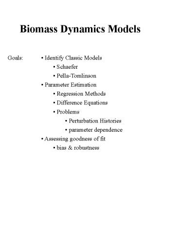
Goals

• Identify Classic Models
• Schaefer
• Pella-Tomlinson
• Parameter Estimation
• Regression Methods
• Difference Equations
• Problems
• Perturbation Histories
• parameter dependence
• Assessing goodness of fit
• bias robustness

2
Overview

• A.K.A. Surplus Production Models
• simple (3 or 4 parameters)
• no age structure
• no time lag
• no immigration/emmigration

• Useful when
• age structure is unavailable
• age related parameters are poorly known

3
The Basic Concept
Bt1 Bt Rt Gt - Mt - Ct
B stock size R recruitment G growth M
natural mortality C catch (fishing mortality)
production R G surplus R G - M Bt1
Bt surplus - Ct surplus Bt1 - Bt Ct
4

• peaks at intermediate biomass
• use actual stock size if available
• commonly, only index of abundance available

5
Schaefer
dB/dt rB(1 - B/K) -C C qEB
r intrinsic rate of population growth K
carrying capacity B biomass E effort q
catchability

• Variables C, E, B
• Parameters r, k, q
• surplus maximum at K/2
• MSY rK/4, EMSY r/2q

6
Pella and Tomlinson
dB/dt rB - rBm/K -C C qEB

• Parameters r, k, q, and m (shape)
• MSY peak is moved by m

7
Difference Equation Forms

• similar properties at low r values
• potential chaotic behavior at large r values

8
Parameter Estimation
I. Equilibrium Methods

• assume dynamics always at equilibrium
• Catch and Surplus at equilibrium
• dB/dt surplus - catch 0

dB/dt 0 rB(1 - B/K) -qEB

• have historical B index, E
• estimate r, k, q, MSY, etc.
• tends to overestimate production Why?

JUST SAY NO!
9
II. Regression Methods

• based upon assumed disequilibrium
• rearrangement of Schaefer model into
  regression form
• Walters Hilborn 1976, Schnute 1977

Bt1 Bt rBt(1-Bt/K) - q BtEt Bt Ut/q
where Ut C/E Ut1/Ut - 1 r - Ut r/kq - qEt
Yt b0 b1 Ut b2 Et
10
III. Time Series Fitting

• Variables C, E, U (C/E)
• Parameters r, k, q and B0
• Fit parameters according to (observed -
  predicted) time series
• U or C can be used
• choice of fitting criteria
• explicit error
• numerical methods required
• C.I. possible by computer intensive methods
• Note at least one more another parameter is
  estimated (error)

11
Perturbation Histories
Yt Ut1/Ut - 1
low CPUElow effort
Ut
high CPUElow effort
Et
low CPUEhigh effort

• different possible histories
• initial high U, low E (over exploitation)
• recoveries (low E, U initially)
• need CONTRAST to estimate regression
  parameters
• odd error assumptions and C.I. s for biomass
  dynamics models

12
PerturbationHistories
Ut1/Ut - 1
Ut
Et

• The one way trip
• exploited to low abundance
• unknown starting point
• little information for management
• Up and Down the Isocline
• increased, then decreased E
• gradual changes
• CPUE correlated with E
• best case, MSY estimated
• cannot distinguish between
• large, low productive
• small, highly productive
• NEED CONTRAST

13

• Estimate r
• low U and low E
• Estimate kq
• high U and low E
• Estimate q
• high E

Ideal Data Rare
MSY rk/4 r/qkq1/4
14
Examining Perturbation HistoriesBy Monte Carlo
Simulation

• Do not know true values in real data
• create a model system
• study the performance of estimators
• controlled numerical conditions

• Generate data from Schaefer Model
• set parameters
• Estimate parameters from new data
• use regression method

r k q MSY True .40 1,000 0.010
100 one way trip .13 290,000 0.003 9245 up
down .39 38,000 0.009 3705 Contrast .47
1,142 0.013 134
15
Assessing Goodness of Fit

• R2 of model
• predicted vs observed
• misleading, high R2 in equilibrium fits!!!
• You should always consider fit relative to
  ALTERNATIVE models
• Also consider parameter bias in the evaluation of
  model performance
• estimators from regression models known to behave
  poorly
• examine via Monte Carlo

16
Auxiliary Information