Simple Linear Regression

1
Simple Linear Regression

• Chapter 3

2
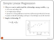
A First-Order (Straight-Line) Model

• where

y Dependent variable (variable to be
modeled sometimes called the response
variable) x Independent variable (variable
used as a predictor of y) E(y) b0 b1x
Deterministic component e (epsilon) Random
error component b0 (beta zero) y-intercept
of the line, i.e., point at which the line
intercepts or cuts through the y-axis (see Figure
3.1) b1 (beta one) Slope of the line,
i.e., the amount of increase (or decrease) in the
mean of y for every 1-unit increase in x (see
Figure 3.1)
3
Steps in Regression Analysis

• Step 1 Hypothesize the form of the model for
  E(y).
• Step 2 Collect the sample data.
• Step 3 Use the sample data to estimate unknown
  parameters in the model.
• Step 4 Specify the probability distribution of
  the random error term, and estimate any unknown
  parameters of this distribution.
• Step 5 Statistically check the usefulness of the
  model.
• Step 6 When satisfied that the model is useful,
  use it for prediction, estimation, and so on.

4
Definition 3.1

• The least squares line is one that satisfies the
  following two properties
• SES(yi -yi)0 i.e., the sum of the residuals is
  0.
• SSES(yi -yi)2 i.e., the sum of the squared
  errors, is smaller than any other straight-line
  model with SE0.

5
Formulas for the Least Squares Estimates

• Slope
• y-intercept
• where

6
Plot of Data
7
Plot of Best Guess
8
Plot of the Least Squares Line
9
Compare the two lines

• Compute SSE for each line
• Line 1 SSE 2
• Line 2 SSE 1.1
• Least Squares line is best

10
Model Assumptions

• Assumption 1 The mean of the probability
  distribution of e is 0. That is, the average of
  the errors over an infinitely long series of
  experiments is 0 for each setting of the
  independent variable x. This assumption implies
  that the mean value of y, E(y), for a given value
  of x is E(y)b0 b1x.
• Assumption 2 The variance of the probability
  distribution of e is constant for all settings of
  the independent variable x. For our straight-line
  model, this assumption means that the variance of
  e is equal to a constant, say, s2, for all values
  of x.
• Assumption 3 The probability distribution of e is
  normal.
• Assumption 4 The errors associated with any two
  different observations are independent. That is,
  the error associated with one value of y has no
  effect on the errors associated with other y
  values.

11
The Probability Distribution of e

• An Estimator of sigma2

12
Estimation of s2 and s for the Straight-Line
(First-Order) Model

• where
• We refer to s as the estimated standard error
  of the regression model.
• Warning When performing these calculations, you
  may be tempted to round the calculated values of
  SSyy, , and SSxy. Be certain to carry at least
  six significant figures for each of these
  quantities to avoid substantial errors in the
  calculation of the SSE.

13
Interpretation of s, the Estimated Standard
Deviation of e

• We expect most (approximately 95) of the
  observed y values to lie within 2s of their
  respective least squares predicted values, .

14
Definition 3.2

• The coefficient of variation is the ratio of the
  estimated standard deviation of e to the sample
  mean of the dependent variable, , measured as a
  percentage

15
Sampling Distribution of

• If we make the four assumptions about e (see
  Section 3.4), then the sampling distribution
  of , the least squares estimator of the slope,
  will be a normal distribution with mean (the
  true slope) and standard deviation

16
A Test of Model Utility Simple Linear Regression

• TWO-TAILED TEST
• Test statistic
• Rejection region
• where t?/2 is based on (n - 2) df
• Assumptions The four assumptions about e listed
  in Section 3.4.

17
A 100(1-a) Confidence Interval for the Simple
Linear Regression Slope b1

• and ta/2 is based on (n-2) df

18
Definition 3.3

• The Pearson product moment coefficient of
  correlation r is a measure of the strength of the
  linear relationship between two variables x and
  y. It is computed (for a sample of n measurements
  on x and y) as follows

19
Warning

• High correlation does not imply causality. If a
  large positive or negative value of the sample
  correlation coefficient r is observed, it is
  incorrect to conclude that a change in x causes a
  change in y. The only valid conclusion is that a
  linear trend may exist between x and y.

20
Definition 3.4

• The coefficient of determination is
• It represents the proportion of the sum of
  squares of deviations of the y values about their
  mean that can be attributed to a linear
  relationship between y and x. (In simple linear
  regression, it may also be computed as the square
  of the coefficient of correlation r.)

21
Practical Interpretation of the Coefficient of
Determination, r 2

• About 100(r 2) of the sample variation in y
  (measured by the total sum of squares of
  deviations of the sample y values about their
  mean ) can be explained by (or attributed to)
  using x to predict y in the straight-line model.

22
Using the Model for Estimation and Prediction
23
A 100(1-a) Confidence Interval for the Mean
Value of y for xxp

• (Estimated standard deviation of )
• or
• where ta/2 is based on (n 2) df

24
A 100(1-a) Prediction Interval for an Individual
y for xxp

• Estimated standard deviation of
• or
• where ta/2 is based on (n 2) df

25
Caution

• Using the least squares prediction equation to
  estimate the mean value of y or to predict a
  particular value of y for values of x that fall
  outside the range of the values of x contained in
  your sample data may lead to errors of estimation
  or prediction that are much larger than expected.
  Although the least squares model may provide a
  very good fit to the data over the range of x
  values contained in the sample, it could give a
  poor representation of the true model for values
  of x outside this region.

26
Comparison of Widths of 95 Confidence and
Prediction Intervals
27
Steps to Follow in a Simple Linear Regression
Analysis

• The first step is to hypothesize a probabilistic
  model. In this chapter, we confined our attention
  to the first-order (straight-line) model
• The second step is to collect the (x,y) pairs for
  each experimental unit in the sample.
• The third step is to use the method of least
  squares to estimate the unknown parameters in the
  deterministic component, b0b1x. The least
  squares estimates yield a model
  with a sum of squared errors (SSE) that is
  smaller than the SSE for any other straight-line
  model.

28
Continued

• The fourth step is to specify the probability
  distribution of the random error component e.
• The fifth step is to assess the utility of the
  hypothesized model. Included here are making
  inferences about the slope b 1, intercepting the
  coefficient of correlation r, and intercepting
  the coefficient of determination r 2.
• Finally, if we are satisfied with the model, we
  are prepared to use it. We can use the model to
  estimate the mean y value, E(y), for a given x
  value and to predict an individual y value for a
  specific value of x.