Simple Linear Regression - PowerPoint PPT Presentation
Title:
Simple Linear Regression
Description:
Simple Linear Regression Often we want to understand the relationships among variables, e.g., SAT scores and college GPA car weight and gas mileage – PowerPoint PPT presentation
Number of Views:143
Avg rating:3.0/5.0
Title: Simple Linear Regression
1
Simple Linear Regression
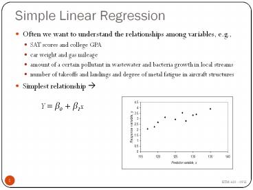
- Often we want to understand the relationships
among variables, e.g., - SAT scores and college GPA
- car weight and gas mileage
- amount of a certain pollutant in wastewater and
bacteria growth in local streams - number of takeoffs and landings and degree of
metal fatigue in aircraft structures - Simplest relationship ?
- Y ß0 ß1x
1
ETM 620 - 09U
2
Example
- An electric power cooperative is concerned about
the cost of power outages in the winter and the
analyst has an idea that these costs are directly
related to the average temperature during the
outage period. A random sampling of power outages
over a number of years was conducted and the cost
per 100 homes (adjusted for inflation) was
determined, with these results
Temp, F Cost/ Outage
45 3,639
42 4,111
44 3,928
37 4,252
33 5,020
45 3,838
35 4,293
38 4,244
39 4,227
40 4,111
30 5,335
2
ETM 620 - 09U
3
Estimating the regression coefficients
- Method of Least Squares
- Determine estimates for ß0 and ß1 so that the sum
of the squares of the residuals is minimized,
that is - Solution to the minimization gives
3
ETM 620 - 09U
4
For our example,
Sample Temp, x Cost, y xiyi xi2
1 45 3,639 163,755 2025
2 42 4,111 172,662 1764
3 44 3,928 172,832 1936
4 37 4,252 157,324 1369
5 33 5,020 165,660 1089
6 45 3,838 172,710 2025
7 35 4,293 150,255 1225
8 38 4,244 161,272 1444
9 39 4,227 164,853 1521
10 40 4,111 164,440 1600
11 30 5,335 160,050 900
sum 428 46998 1805813 16898
4
ETM 620 - 09U
5
What does this mean?
- We can draw the regression line that describes
the relationship between temperature and outage
cost - We can also predict the cost of outages based on
expected temperatures.
5
ETM 620 - 09U
6
Dangers of regression analysis
- You can regress any variable on any other
variable - e.g., hair loss and heart disease hours playing
video games and number of arrests for violent
behavior consecutive hours in class and
retention of material etc. - Which of these relationships can you legitimately
claim reflect a causal relationship between the
predictor and the response? - The regression equation is a best fit for the
data on which it is based, but may lose validity
for predictor values outside the range of the
data. - For example, our outage cost data implies that
the cost per outage decreases as the temperature
increases do you believe that temperatures in
the 80s or 90s will result in low-cost outages?
7
How good is our prediction?
- Estimating the variance
- Lack of fit test,
- Tests the hypotheses
- H0 the model adequately fits the data
- H1 the model does not fit the data
- As with our goodness-of-fit tests, a high p-value
indicates that the model is adequate.
7
(see next page)
ETM 620 - 09U
8
How good is our prediction?
- Coefficient of determination, R2
- a measure of the quality of fit, or the
proportion of the variability explained by the
fitted model. - Use with care increasing the number of
variables will usually increase R2, but this
doesnt necessarily make it a better model!
ETM 620 - 09U
8
9
Linear regression in Excel
- Step 1 Graph the data
- Does it look like a straight line is the best
fit?
9
ETM 620 - 09U
10
Step 2 Perform the analysis
- Choose Regression from the Data Analysis menu
(under Tools). Input the Y-range (Cost, including
the label) and X-range (Temp, including the
label), then select - Labels if you included those in your data
range. - Your desired location for the output.
- Residuals and Normal Probability Plot, as
desired. - Choose OK
10
ETM 620 - 09U
11
Step 3 Check assumptions
- Look at residuals plot and normal probability
plots.
11
ETM 620 - 09U
12
Step 4. Evaluate the results.
12
ETM 620 - 09U
13
Step 5. Specify and use the model.
- Simple linear model
- Use the model to
- Make predictions
- expected costs
- budgeting
- Recommend actions
- identify and address sources of cost increase
13
ETM 620 - 09U
14
In Minitab
- Step 1 Graph the data (for one or two predictor
variables)! - Again, do you think a simple linear relationship
is the best fit? - Step 2 Select Stat ? Regression ?Regression
- Step 3 Choose Response (y) and Predictor
(x). - Step 4 In Options, check the Lack of Fit
box. (Fit Intercept box should be checked by
default.) Click OK. - Step 6 In Graphs select the appropriate
residual plots to create. - Step 5 Click OK.
- Step 6 Evaluate the residual plots and results.
14
ETM 620 - 09U
15
Transformation to a straight line ..,
- If simple linear regression is not appropriate
because the underlying function is nonlinear,
then we have two choices - fit a more complex model
- transform the model to a straight-line model
- Simplest transformation logarithmic
transformation - Original model
- Transformed model


