Simple Regression - PowerPoint PPT Presentation

1 / 40
Title:
Simple Regression
Description:
Chart/Add Trendline/Linear/Display equation, R2. Menu ... Find mother's height = 60', find average daughter's height. Repeat for mother's height = 62', 64' ... – PowerPoint PPT presentation
Number of Views:32
Avg rating:3.0/5.0
Title: Simple Regression
1
Simple Regression
- In confidence intervals and hypothesis testing,
we examined a single parameter of one variable - In chi-square analysis, we also can test for the
existence of a relationship between two variables - In regression analysis, we also can determine the
strength of the relationship between two or more
variables, build models, and make predictions - We will begin with a fairly complete description
of two-variable models before moving to multiple
regression and logistic regression
2
The Linear Model
- The simplest relationship between two variables
is a linear one - y ? ?x
- x independent or explanatory variable (cause)
- y dependent or response variable (effect)
- intercept (value of y when x 0)
- ? slope (change in y when x increases one unit)
- Before beginning a regression, think about
whether a linear relationship is reasonable
3
The Error Term
- Linear relationships are rarely precise
measure-ment error and inherent variability
result in a distribution of values of y for a
given value of x. - We represent this variability with an error term,
? - y ? ?x ?
- where ? is normally distributed random variable,
with a mean of 0 and a standard deviation of ?
(constant, independent of xhomoscedasticity). - A plot of P(yx) v. y is a normal distribution
with a mean of ? ?x and a standard deviation of
?.
4
Probability of y for a given value of x
5
(No Transcript)
6
Estimating ?, ?, ? Least Squares
- Based on sample data (xi,yi), choose a and b
(estimates of ? and ?) such that the sum of the
squared residuals is minimized (least squares)
Check that values of a and b make sense!
7
Residuals and Standard Error
- The predicted or best fit value of y for a
given xi is y-hat the difference between y-hat
and the observed value of y is the residual
The key assumption is that the residuals are
independent and normally distributed with a
constant standard deviation
8
Excel Functions
- Scatterplot
- Chart/Add Trendline/Linear/Display equation, R2
- Menu-driven tools
- Tools/Data Analysis/Regression
- Tools/Data Analysis Plus/Stepwise Regression
- Tools/OLS Regression
- Excel functions
- a INTERCEPT(y-range,x-range)
- b SLOPE(y-range,x-range)
- se STEYX(y-range,x-range)
9
Goodness of Fit
- The total variability in y (SST) has two
components - variability explained by the regression (SSR)
- remaining or unexplained variability (SSE)
The proportion of the variability that is
explained by the regression is the coefficient
of determination
10
(No Transcript)
11
(No Transcript)
12
Degree of Linear Correlation
- R2 1 perfect linear correlation R2 0 no
correlation - High R2 good fit only if linear model is
appropriate always check with a scatterplot - Correlation does not prove causation x and y may
both be correlated to a third (possibly
unidentified) variable - A more popular (but less meaningful) measure is
the correlation coefficient
R2 RSQ(y-range,x-range r
CORREL(y-range,x-range)
13
R2 0.67
R2 0.67
R2 0.67
R2 0.67
14
Inferences about the Slope
- The standard error of the slope
Note that sb depends on both se and sx. All else
equal, larger sx produce smaller sb. Confidence
interval ? b t?/2,dfsb df n 2 for one
independent variable. To test the null hypothesis
that ? 0 (i.e., no association between x and
y), find the p value for
15
(No Transcript)
16
Inferences about Correlation
- You can do this same hypothesis test (no
correlation) if you know only r (or R2) and n.
The standard error of r is equal to
It can be shown that
So R2 0.1 is significant (? 0.05) if n gt 40.
17
Significant value of R2 for given n
18
What Does Regression Mean?
19
What Does Regression Mean?
- Draw best-fit line free hand
- Find mothers height 60, find average
daughters height - Repeat for mothers height 62, 64 70 draw
best-fit line for these points - Draw line daughters height mothers height
- For a given mothers height, daughters height
tends to be between mothers height and mean
height regression toward the mean
20
What Does Regression Mean?
21
Prediction
- The value of y predicted by the best-fit line for
a given x is - This prediction is uncertain for two reasons
- The estimated regression line isnt the true
regression line (a ? ?, b ? ?) this uncertainty
is reduced as the sample size, n, is increased - There is natural variability in y for a given
value of x. We model this with a normal
distribution with constant standard deviation ?
se.
22
Uncertainty in Mean Value of y
- If we knew the exact values of ? and ?, there
would be no uncertainty in the mean value of y
for a given value of x (i.e., the best-fit line) - The uncertainty in the mean value (y-hat) that
arises from the uncertainty in a and b is
- This is the error in the location of the best-fit
line - When x 0, (standard error of
intercept)
23
Uncertainty in Individual Predicted Value
- If we knew the exact values of ? and ?, the
uncertainty in any individual value of y would be
given by ? se, regardless of the value of x. - The overall uncertainty, including that arising
from the uncertainty in a and b, is
- Error grows as x moves away from the middle of
the data. Extrapolation (predicting y for x
outside of range of original data) is frowned
upon.
24
Prediction Using Data Analysis Plus
- Enter in the spreadsheet the value of x for which
you would like to calculate y-hat and its
confidence interval - Tools/Data Analysis Plus/Prediction Interval
- Input y range and x range click labels if
appropriate - Input given x range
- Input confidence level, click OK
25
Analysis of Residuals
- Plot the residuals and look for
- Outliers. Check residuals outside 3se. Because
regression minimizes the sum of the squared
residuals, the results are sensitive to outliers,
particularly for extreme values of x.
26
Testing for Outliers
- Compute and inspect standardized residuals
- To see whether a potential outlier observation is
important, delete the case and rerun the
regression - If regression coefficients are basically
unchanged (new values are within the confidence
intervals of the original regression), the
observation is not an important outlier - Otherwise, consider whether there is a reasonable
basis for removing the observation
27
Testing for Non-Normality
- Assumption residuals are normally distributed
- Estimates of regression coefficients are fairly
robust to violations of this assumption
significant violations are usually evidenced by
outliers or other problems with residuals - To inspect visually, make a histogram of the
residuals and check that it is approximately
bell-shaped and symmetrical - Data Analysis Plus/Chi-Squared Test of Normality
28
Analysis of Residuals
- Non-linearity. The mean value of the residuals
should be zero, independent of x. If residuals
exhibit a curved pattern, a non-linear model may
be more appropriate.
29
Testing for Non-Linearity
- Visual inspection is usually sufficient
- Right click on data in residual plot, select add
trendline, select second-order polynomial
(quadratic), include R2 on chart - If R2 is large (e.g., gt 4/(n2)), then curvature
is significant consider a non-linear
transformation
30
Analysis of Residuals
- Heteroscedasticity. The standard deviation, se,
should be constant, independent of x. If the
spread of residuals increases with x, a
logarithmic model may be appropriate.
31
Testing for Heteroscedasticity
- Visual inspection is usually sufficient
- In professional statistics programs (SPSS,
STATA), use the Cook-Weisburg test - Otherwise, split data into two parts
do hypothesis test to compare the
average residuals for each part
32
Analysis of Residuals
- Autocorrelation. The residuals should be random
and uncorrelated. If there a regular pattern in
the residuals (e.g., up-down-up-down), common in
time-series data, dummy, lagged, or difference
variables may be needed.
33
Testing for Autocorrelation
- First-order autocorrelation test for correlation
between et and et1 - Second-order (et and et2), third-order, etc.
- Durbin-Watson Test
- D ? 2 2r
- If no autocorrelation, D ? 2
- If strong positive autocorrelation, D ? 0
- If strong negative autocorrelation, D ? 4
- Critical value of D depends on n, ?, k
34
Transformations
- Transformations are used for three main reasons
- to linearize non-linear relationships between
independent and dependent variables - to produce residuals that are normally
distributed with constant standard deviation - to remove autocorrelation from a time series
- We will focus on the first two. No information is
lost in transformations, but care must be taken
in interpreting the coefficients, and the
transformed model must be validated.
35
Exponential Function
- y aebx linearize by regressing log(y) on x
- Use if a unit change in x produces a fixed
percentage change in y - Most common in time series, when y grows at a
constant rate (b percent per year)
36
Power Function
- y axb linearize by regressing log(y) on log(x)
- Use if a one percent change in x produces a fixed
percentage change in y slope is elasticity - Also used to stabilize variance
- Convenient if y is product of several factors
37
Logarithmic Function
- y a blog(x) regress y on log(x)
- Use if a one percent change in x produces a fixed
change in y - Also used to stabilize variance
38
Other Transformations
- Polynomial mostly used to improve fit
- y a b1x b2x2 define x2 x2 and regress
- y a b1x b2x2
- Poisson used if y counts, to stabilize variance
Binomial used y proportion, to stabilize
variance
Logistic used to model populations, resources
39
Weighted Least Squares
- Least squares regression model assumes errors are
normally distributed with constant variance - Sometimes we can correct for heteroscedasticity
with transformationse.g, log(y) instead of y - Sometimes each y has a different measurement
error, or each y represents a different sized
population. In this case we can use weighted
least squares, in which each case is given a
different weight in determining the best-fit
line. Unfortunately, Excel does not include
weighted least squares.
40
(No Transcript)
Recommended
CrystalGraphics Presentations